Download
1 / 43
430 likes | 515 Views
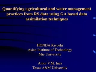
Data Assimilation using Remote Sensing and Genetic Algorithms: Applications to Agriculture and Water Management. Amor V.M. Ines and Kyoshi Honda Space Technology Applications and Research, School of Advanced Technologies Asian Institute of Technology (AIT), Bangkok, Thailand. Introduction.

E N D
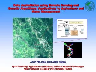
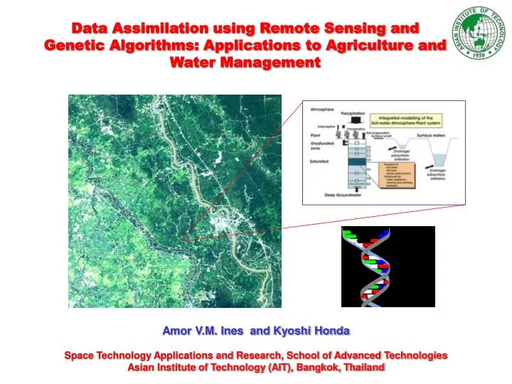
Data Assimilation using Remote Sensing and Genetic Algorithms: Applications to Agriculture and Water Management Amor V.M. Ines and Kyoshi Honda Space Technology Applications and Research, School of Advanced Technologies Asian Institute of Technology (AIT), Bangkok, Thailand
Introduction Regional studies in agricultural and water management require a large amount of spatial and temporal information. Remote sensing (RS) and geographic information system (GIS) have been used to account for the spatial information. Temporal integration with RS is quite difficult and expensive especially with high spatial resolution data. This gap can be bridged upon by the integration of RS/GIS with physically based simulation models, which is now becoming a robust approach in water management studies. But a major problem to be overcome is the derivation of the spatial and temporal data requirements of simulation models, which are mostly non-observable from RS data, e.g. soil hydraulic properties and other transport parameters, sowing dates, water management practices etc.
Objectives We aim to present a methodology in quantifying irrigation water management from remote sensing (RS) based on data assimilation technique. A methodology for high spatial resolution RS data (HSRD) based on stochastic approach and a recently developed procedure for low spatial resolution (LSRD) where the issue of mixed-pixel in agriculture is addressed are presented in this seminar. For the HSRD methodology, results of a case study in an irrigation system in Kaithal, Haryana, India is presented. The LSRD methodology is demonstrated using synthesized “RS data” for a hypothetical pixel. The issue of computational efficiency and how it has been improved is also discussed.
Data Assimilation using RS and GA 4 . 00 4 . 00 3 . 00 3 . 00 2 . 00 2 . 00 ET / LAI 1 . 00 1 . 00 0 . 00 0 . 00 0 45 90 135 180 225 270 315 360 0 45 90 135 180 225 270 315 360 Set of Parameters Water management, sowing date, soil property and etc. RS Observed - SWAP Physical Model - e.g SEBAL Analysis Fitting ET / LAI Assimilation by finding set of parameters By Genetic Algorithms Day Of Year Day Of Year RS Modeling
[x, y] Irrigation dates, depths Spatial distribution yield t+2t t+t ETa water balance Extended SWAP RS model SEBAL By Genetic Algorithm water productivity . . . t t+2t … t+t t+nt Past Time The future Stochastic parameter estimation technique
Soil-Water-Atmosphere-Plant Model (SWAP) Adopted from Van Dam et al. (1997) Drawn by Teerayut Horanont (AIT)
Extended SWAP model μi, σi Etc… Spatial representation of the system
Surface Energy Balance Algorithm for Land (SEBAL) Adopted from WaterWatch Drawn by Teerayut Horanont (AIT)
Surface Energy Balance Algorithm for Land (SEBAL) Rn = K – K + L – L Energy Balance Equations Rn = H + G + λET Rn – Net radiation H – Sensible heat flux G – Soil heat flux λET – Latent heat flux K – incoming and outgoing shortwave radiation L – incoming and outgoing longwave radiation Units in W m-2
eaten eaten Just married eaten eaten eaten down to hole A Practical Genetic Algorithms low IQ high jumpers high IQ low jumper low IQ low jumpers gluttons
A1 B5 B1 Selection Reproduction Crossover Mating Pool A5 B1 B5 Mutation . : Genetic Algorithm in a nutshell Variable1 Variable2 Fitness (Measure) A1 B1 : (t+1) Population (t) . An Bn A3
February 4, 2001 March 8, 2001 ETa, mm ETa, mm 2.90 2.48 2.06 1.64 1.22 4.20 m m 0.80 3.44 2.68 1.92 1.16 0.40 ETa in Bata Minor, Kaithal, Haryana, India Results from SEBAL Analysis
Cropped area delineation Cropped area Cropped area February 4, 2001 March 8, 2001
Fitness Function Water management variables (Irrigation scheduling criterion) Depth to groundwater k = {μα, σα, μn, σn, μTa/Tp, σTa/Tp, μeDate, σeDate, μgw, σgw, μwq, σwq} crop management variables (Emergence dates - represent the sowing dates) Water quality (Salinity) Soil hydraulic properties (Mualem-Van Genuchten parameters)
GA solution to the regional inverse modeling February 4, 2001 March 8, 2001
System characteristics derived by GA Derived System characteristics from IM_GA * Mualem-Van Genuchten (MVG) parameters. ** Sowing dates were represented by emergence dates in Extended SWAP. ***Irrigation scheduling criterion, Ta/Tp **** Average value of surface water and groundwater, surface water has good quality for irrigation + Assumed spatially distributed but not significantly distributed in time
Data Collected IM_GA Sandy Clay Loam Validation Emergence dates: Mean: Nov 23; SD: 8 days Soil water retention curve
Groundwater depths Average groundwater salinity levels in Bata Minor Irrigation depths: Measured: 180-485 mm Predicted: 125-572 mm
Measured and estimated agro-hydrological variables. Note: Irrigation (mm); Yield (kg ha-1); PW (kg m-3); Ir, ETa and Ta (mm); cv is coefficient of variation.
A typical mixed-pixel problem in agriculture Time … - Time series RS data - Sub-pixel information 1.1 x 1.1 km2 Depending on the proportions of rainfed1, irrigated2 and irrigated3 in the 1.1 km x 1.1 km pixel
A simple mixed-pixel model Assuming that: (1) (2) (3) (4) Objective Function: Simulation model RS data (5) Where: (6)
A simple mixed-pixel model Subject to these constraints: Possible range of sowing dates: Constraints to avoid cropping overlaps: (7) (13) (8) (14) (9) (15) Proportions of cropping area: (10) (16) (11) Possible range of cropping area: (12) (17) (18) (19)
Modified Penalty Approach (20) (21) Penalties: GA (22) (23) (24) (26) (25) The chromosomes consisted only of 8 genes because A3 can be expressed in terms of A1 and A2 i.e. A3=|1-A1-A2| hence the length of string is reduced. The chromosome (p) then for this problem is defined as:
Solution Approaches A. Dynamic Linkage Approach B. Look up table Approach
- Look up table - 4 . 00 3 . 00 4 . 00 2 . 00 3 . 00 2 - m 1 . 00 2 2 . 00 LAI, m 0 . 00 1 . 00 0 45 90 135 180 0 . 00 0 45 90 135 180 225 270 315 360 Day Of Year Look up table Un-mixing algorithm Set of Parameters Water management, sowing date, area fractions and etc. RS Observed - SWAP Physical Model - Minimized 2 - m 2 LAI, m Assimilation by finding set of parameters using GA 225 270 315 360 Day Of Year Dynamic Linkage
GA solutions to the mixed-pixel problem (dynamic linkage) Note: sdk,j in Day Of Year (DOY) where sd = sowing date; k = r (rainfed), i2 (irrigated with two-croppings), i3 (irrigated with three croppings); j = 1 (first sowing), 2 (second sowing),3 (third sowing); ak = is the area fraction of k.; 10d = aggregated every 10 days;10dave = moving average every 10 days. †population = 10 and 5, respectively; prob.crossover=0.5; prob.mutation (creep)=0.5; seed=-1000;no. of generation=150. ‡ population = 5 for both cases; genetic parameters same as ET. Link
Results using ET data every 10 days (ET10dE): at 10% level of error Dynamic Linkage Results using ET data every 10 days (ET10daveE): at 10% level of error
GA solutions to the mixed-pixel problem with water management (dynamic linkage) Note: w2 = is the water management variable (defined as the irrigation scheduling criteria, Ta/Tp) for i2. w3= is the water management variable (defined as the irrigation scheduling criteria, Ta/Tp) for i3.
Conclusions Data assimilation using RS is very promising in agriculture and water management studies. The methodology developed for HSRD proves to be useful in understanding the processes of a hydrologic system as a whole. Processes that are hard to measure in the field can be analyzed using simulation models. It has been known that LRSD can provide a vast of spatial information especially if the sub-pixel information contained in the large pixel can be abstracted. This mixed-pixel problem is a usual bottleneck in using LSRD for agricultural and water management studies. Based on our numerical experiments, solution of the mixed-pixel problem in agriculture is highly possible using the proposed approach for LSRD. Overall, GA is powerful in both HSRD and LSDR data assimilation.
Future Works Application of the LSRD methodology using actual data Data assimilation using high and low resolution data