Download
1 / 84
840 likes | 860 Views
Explore the concept of Optical Flow and its applications in motion extraction, tracking, and analysis. Learn about the mathematical formulations, algorithms, and challenges in detecting motion patterns in images and videos. Discover how Optical Flow plays a crucial role in various fields such as surveillance, autonomous driving, and gesture analysis. Enhance your knowledge of motion segmentation and feature tracking for 3D reconstruction through this comprehensive overview.

E N D
Motion Extraction
Motion is a basic cue Motion can be the only cue for segmentation Biologically favoured because of camouflage
Motion is a basic cue … which set in motion a constant, evolutionary race, encouraging animals to sit still, only moving in bursts
Motion is a basic cue Motion can be the only cue for segmentation
Motion is a basic cue Even impoverished motion data can elicit a strong percept http://www.biomotionlab.ca/Demos/BMLwalker.html
Some applications of motion extraction • Change / shot cut detection • Surveillance / traffic monitoring • Autonomous driving • Analyzing game dynamics in sports • Motion capture / gesture analysis (HCI) • Image stabilisation • Motion compensation (e.g. medical robotics) • Feature tracking for 3D reconstruction • Etc.!
Shot cut detection & Keyframes Shot cut Shot cut
3D: Structure-from-Motion Tracked Points gives correspondences
3D: Structure-from-Motion Temple of the Masks, Edzna, Mexico
in this lecture... Several techniques, but… this lecture is restricted to the 1. detection of the “optical flow” 2. tracking with the “Condensation filter”
Definition of optical flow Ideally, the optical flow is the projection of the 3D velocity vectors onto the image A motion vector is sought at every pixel of the image OF = apparent motion of brightness patterns In practice
OF may fail to capture the real motion ! Two examples : 1. Uniform, rotating sphere ⇓ O.F. = 0 2. No motion, but changing lighting ⇓ O.F. ≠ 0
Qualitative formulation Suppose a point of the scene projects to a certain pixel of the current video frame. Our task is to figure out to which pixel in the next frame it moves… That question needs answering for all pixels of the current image. In order to find these corresponding pixels, we need to come up with a reasonable assumption on how we can detect them among the many. We assume these corresponding pixels have the same intensities as the pixels the scene points came from in the previous frame. That will only hold approximately…
Mathematical formulation I (x,y,t) = brightness at (x,y) at time t Optical flow constraint equation : This equation states that if one were to track the image projections of a physical point through the video, it would not change its intensity… This tends to be true over short lapses of time. (Note the different types of time derivatives!)
Mathematical formulation We will use as shorthand notation for
The aperture problem Note that we can measure the 3 derivatives of I, but that u and vare unknown 1 equation in 2 unknowns
The aperture problem Aperture problem : only the component along the gradient can be retrieved
Remarks 1. The underdetermined nature could be solved using higher derivatives of intensity 2. for some intensity patterns, e.g. patches with a planar intensity profile, the aperture problem cannot be resolved anyway. For many images, large parts have planar intensity profiles… higher-order derivatives than 1st order are typically not used (also because they are noisy)
Horn & Schunck algorithm Breaking the spell via an … additional smoothness constraint : to be minimized, besides the OF constraint equation term minimize es+λec (also reduces influence of noise)
The calculus of variations look for functions that extremize functionals (a functional is a function that takes a vector as its input argument, and returns a scalar) like for our functional: what are the optimal u(x,y) and v(x,y) ?
and The calculus of variations look for functions that extremize functionals with ,
Calculus of variations Suppose 1. f(x) is a solution 2. η(x) is a test function with η(x1)= 0 and η(x2) = 0 We then consider Rationale: supposed f is the solution, then any deviation should result in a worse I; when applying classical optimization over the values of the scalarethe optimum should be e = 0
Calculus of variations Suppose 1. f(x) is a solution 2. η(x) is a test function with η(x1)= 0 and η(x2) = 0 We then consider With this trick, we reformulate an optimization over a function into a classical optimization over a scalar…a problem we know how to solve
Calculus of variations Suppose 1. f(x) is a solution 2. η(x) is a test function with η(x1)= 0 and η(x2) = 0 for the optimum : Around the optimum, the derivative should be zero
Calculus of variations Suppose 1. f(x) is a solution 2. η(x) is a test function with η(x1)= 0 and η(x2) = 0 for the optimum : with with
Using integration by parts : Calculus of variations Using integration by parts: where
Calculus of variations Using integration by parts :
Using integration by parts : Therefore Calculus of variations regardless ofη(x), then Euler-Lagrange equation
1. Simultaneous Euler-Lagrange equations, i.c. one for u and one for v : • 2. 2 independent variables x and y Calculus of variations Generalizations
Hence Now by Gauss’s integral theorem, such that Calculus of variations = 0
Calculus of variations Consequently, for all test functions η , thus is the Euler-Lagrange equation
so the Euler-Lagrange equations are is the Laplacian operator Horn & Schunck The Euler-Lagrange equations : In our case ,
Horn & Schunck Remarks : 1. Coupled PDEs solved using iterative methods and finite differences (iteration i) i i 2. More than two frames allow for a better estimation of It 3. Information spreads from edge- and corner-type patterns
Horn & Schunck, remarks 1. Errors at object boundaries 2. Example of regularisation (selection principle for the solution of ill-posed problems by imposing an extra generic constraint, like here smoothness)
condensation filter as an example of a `tracker’, shifting the emphasis from pixels to objects…
Condensation tracker System. M. Measur. M. state vector noise in system model observation vector noise in measurement model
1. Prediction , based on the system model ( f = system transition function) 2. Update , based on the measurement model ( h = measurement function) is the history of observations Condensation tracker
position velocity Condensation tracker Example System model Measurement model
Condensation tracker Recursive Bayesian filter Object not as a single state but a prob. distribution
1. Prediction 2. Update Condensation tracker Recursive Bayesian filter Object not as a single state but a prob. Distribution (p here means probability…)
1. Prediction 2. Update can be considered a normalization factor Condensation tracker Recursive Bayesian filter Object not as a single state but a prob. distribution