Atmospheric Sounding Visualization
250 likes | 277 Views
Atmospheric Sounding Visualization. Sancho McCann.

Atmospheric Sounding Visualization
E N D
Presentation Transcript
Atmospheric Sounding Visualization Sancho McCann Permission is granted to copy, distribute and/or modify this document under the terms of the GNU Free Documentation License, Version 1.2 or any later version published by the Free Software Foundation; with no Invariant Sections, no Front-Cover Texts, and no Back-Cover Texts. A copy of the license is available at http://www.gnu.org/licenses/gpl.txt
Soundings • Pressure • Altitude • Temperature • Moisture • Wind Speed • Wind Direction
Meteorology 101 • At 100% humidity, the temperature has reached the dewpoint
Meteorology 101 • Lifting causes cooling at 9.8ºC per 1000m
Meteorology 101 • Inside a cloud, the temperature decreases much more slowly ~ 6º per 1000m
Sample Sounding Data 72694 SLE Salem Observations at 12Z 08 Oct 2006 ----------------------------------------------------------------------------- PRES HGHT TEMP DWPT RELH MIXR DRCT SKNT THTA THTE THTV hPa m C C % g/kg deg knot K K K ----------------------------------------------------------------------------- 1020.0 61 6.0 3.8 86 4.95 0 0 277.6 291.2 278.4 1000.0 224 10.0 6.9 81 6.28 15 4 283.1 300.7 284.2 997.0 249 10.2 7.1 81 6.38 17 5 283.6 301.5 284.7 990.3 305 10.0 6.8 80 6.30 20 6 284.0 301.6 285.0 954.6 610 9.0 5.2 77 5.83 25 9 286.0 302.6 287.0 925.0 871 8.2 3.8 74 5.46 5 12 287.7 303.4 288.6 920.2 914 8.1 4.0 75 5.56 5 12 288.0 304.0 289.0 909.0 1015 7.8 4.4 79 5.80 2 14 288.7 305.4 289.7 902.0 1079 8.8 -11.2 23 1.81 360 15 290.4 296.0 290.7
Problems • Easy to forget • Easy to make mistakes • Difficult to compare • Information doesn’t pop out
Informal Evaluation • 2 Students • Given instruction on the AtmosView • Given a set of questions to answer • Given instruction on the Skew-T • Given a set of questions to answer
Strengths • Successful improvement to Skew-T • Data pops out • Quick comparisons • Useable in miniature • Not reliant on colour
Areas for Improvement • Temperature not displayed
Future Work • Improve usability of system • Target audience: amateur meteorologists (glider pilots, students, storm-chasers)