Download
1 / 15
180 likes | 577 Views
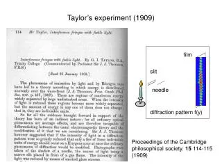
Taylor’s experiment (1909). film. slit. needle. diffraction pattern f(y). Proceedings of the Cambridge philosophical society. 15 114-115 (1909). Taylor’s experiment (1909). Interpretation: Classical: f(y) <E 2 (y)>

E N D
Taylor’s experiment (1909) film slit needle diffraction pattern f(y) Proceedings of the Cambridge philosophical society. 15 114-115 (1909)
Taylor’s experiment (1909) Interpretation: Classical: f(y) <E2(y)> Early Quantum (J. J. Thompson): if photons are localized concentrations of E-M field, at low photon density there should be too few to interfere. Modern Quantum: f(y) = <n(y)> = <a+(y)a(y)> <E-(y)E+(y)> E+(r) = a exp[i k.r – iwt] E-(r) = a+ exp[-i k.r + iwt] f(y) same as in classical. Dirac: “each photon interferes only with itself.” film slit needle diffraction pattern f(y)
Hanbury-Brown and Twiss (1956) Nature, v.117 p.27 Correlation g(2) Tube position I Detectors view same point t I Detectors view different points Signal is: g(2) = <I1(t)I2(t)> / <I1(t)><I2(t)> t
Signal is: g(2) = <I1I2> / <I1><I2> = < (<I1>+dI1>) (<I2>+dI2>) > / <I1><I2> Note: <I1> + dI1≥ 0 <I2> + dI2 ≥ 0 <dI1> = <dI2> = 0 g(2) = (<I1><I2>+<dI1><I2>+<dI2><I1>+<dI1dI2>)/<I1><I2> = 1 + <dI1dI2>)/<I1><I2> = 1 for uncorrelated <dI1dI2> = 0 ≥ 1 for positive correlation <dI1dI2> = 0 e.g. dI1=dI2 ≤1 for anti-correlation <dI1dI2> < 0 Classical optics: viewing the same point, the intensities must be positively correlated. Hanbury-Brown and Twiss (1956) Correlation g(2) Tube position I Detectors view same point t I Detectors view different points I1= I0/2 I0 t I2= I0/2
Kimble, Dagenais + Mandel 1977 PRL, v.39 p691 Correlation g(2) Classical: correlated I1= I0/2 I0 I2= I0/2 t1 - t2 Correlation g(2) Quantum: anti-correlated n1=0 or 1 n0=1 n2= 1- n1 t1 - t2
Kimble, Dagenais + Mandel 1977 PRL, v.39 p691
Kimble, Dagenais + Mandel 1977 PRL, v.39 p691 Interpretation: g(2)(t) < a+(t)a+(t+t)a(t+t)a(t)> < E-(t) E-(t+t) E+(t+t)E+(t)> E+(t) = a exp[i k.r – iwt] E-(t) = a+ exp[-i k.r + iwt] Pe time t
Pelton, et al. 2002 InAs QD relax fs pulse emit
Pelton, et al. 2002 Goal: make the pure state |> = a+|0> = |1> Accomplished: make the mixed state r 0.38 |1><1| + 0.62 |0><0|
Holt + Pipkin / Clauser + Freedman / Aspect, Grangier + Roger 1973-1982 J=0 J=1 J=0 Total angular momentum is zero. For counter-propagating photons implies a singlet polarization state: |> =(|L>|R> - |R>|L>)/2
Holt + Pipkin / Clauser + Freedman / Aspect, Grangier + Roger 1973-1982 Total angular momentum is zero. For counter-propagating photons, implies a singlet polarization state: |> =(|L>|R> - |R>|L>)/2 |> = 1/2(aL+aR+ - aR+aL+)|0> = 1/2(aH+aV+ - aV+aH+)|0> = 1/2(aD+aA+ - aA+aD+)|0> Detect photon 1 in any polarization basis (pA,pB), detect pA, photon 2 collapses to pB, or vice versa. If you have classical correlations, you arrive at the Bell inequality -2 ≤ S ≤ 2.
Holt + Pipkin / Clauser + Freedman / Aspect, Grangier + Roger 1973-1982 a b a' 22.5° b' |SQM| ≤ 22 = 2.828...