Download
1 / 43
430 likes | 530 Views
Learn the basics of genetic algorithms, simulating evolution to optimize solutions. Understand selection, crossover, and mutation operators. Maximize fitness functions with practical examples.

E N D
15.053 Tuesday, May 14 • Genetic Algorithms Handouts: Lecture Notes Question: when should there be an additional review session?
The basic genetic algorithm • Developed by John Holland in 1975 • Simulates the process of evolution • Basic Principle: Evolution can be viewed as • an optimizing process
More on physical analogies • Physical Analogies as a guiding principle • for optimization problems • – Genetic Algorithms • • John Holland 1975 • – Simulated Annealing • • Kirkpatrick • – Ant Colony Systems
The basic genetic algorithm • Loosely modeled on natural selection with a touch • of molecular biology thrown in. • Fitter individuals mate [selection operator]. • The chromosomes of each child are formed as a • mixture of the chromosomes of the parents • [crossover operator]. • Mutation adds diversity within the species and a • greater scope for improvement [mutation operator]. • Chromosomes encode the relevant information.
GA terms chromosome (solution) gene alleles (variable) (values) selection crossover mutation population Objective: maximize fitness function (objective function)
Selection Operator: Selects two parents from the population for mating. The selection is biased towards fitter individuals. Crossover Operator: Each child is obtained as a random mixture of its parents using a crossover operation. Mutation Operator: At times an individual in the population undergoes a random mutation.
A Simple Example: Maximize the number of 1’s • Initial Population Fitness • 1 1 1 0 1 4 • 0 1 1 0 1 3 • 0 0 1 1 0 2 • 1 0 0 1 1 3 • Average fitness 3 • Usually populations are much bigger, • say around 50 to 100, or more.
Crossover Operation: takes two solutions and creates a child (or more) whose genes are a mixture of the genes of the parents. Select two parents from the population. This is the selection step. There will be more on this later. parent 1parent 2 0 1 1 0 1 1 0 0 1 1
Crossover Operation: takes two solutions and creates a child (or more) whose genes are a mixture of the genes of the parents. 1 point crossover: Divide each parent into two parts at the same location k (chosen randomly.) parent 1parent 2 0 1 1 0 1 1 0 0 1 1 Child 1 consists of genes 1 to k-1 from parent 1 and genes k to n from parent 2. Child 2 is the “reverse”. child 1 child 2 0 1 1 1 1 1 0 0 0 1
Selection Operator • Think of crossover as mating • Selection biases mating so that fitter • parents are more likely to mate. For example, let the probability of selecting member j be fitness(j)/total fitness Example: 1. 1 1 1 0 1 4 2. 0 1 1 0 1 3 3. 0 0 1 1 0 2 4. 1 0 0 1 1 3 Total fitness 12 Prob(1) = 4/12 = 1/3 Prob(3) = 2/12 = 1/6
Example with Selection and Crossover Only original after 5 after 10 generations generations 1 0 0 1 1 1 1 0 1 1 1 1 0 1 1 0 1 0 0 0 1 0 1 1 1 1 0 0 1 1 0 0 0 0 1 1 1 0 1 1 1 1 0 1 1 1 1 1 1 1 1 1 0 1 1 1 1 0 1 1 . . . 0 0 1 0 0 1 1 0 1 1 1 1 0 1 1 1 1 0 1 1 1 1 0 1 1 1 1 0 1 1 2.8000 3.7000 3.9000
Mutation • Previous difficulty: important genetic • variability was lost from the population • Idea: introduce genetic variability into the • population through mutation • simple mutation operation: randomly flip • q% of the alleles (bits) in the population.
Previous Example with a 1% mutation rate original after 5 after 10 generations generations 1 0 0 1 1 1 1 0 1 1 1 1 1 1 1 0 1 0 0 0 1 1 1 1 1 1 1 1 1 1 0 0 0 0 1 1 1 1 1 1 1 1 1 1 1 1 1 1 1 1 1 1 1 1 1 1 1 1 1 1 . . . 1 0 0 0 1 0 1 1 1 1 1 1 1 1 1 0 0 1 0 0 1 1 1 1 1 1 1 1 1 1 1 1 0 1 1 1 1 1 1 1 1 1 1 1 1 2.8000 4.8000 4.9000
Representations of Operators illustrated on a bit-based representation Selection Crossover Mutation
The basic genetic algorithm • define the representation • – how the solution is • represented • define “fitness” function • – objective function • define the operators • – initialization, crossover, • mutation initialize population select two parents create 1 or 2 children mutate population modify population should we stop or go on? finish
Generation based GAs In generation based GA’s we create children one generation at a time. Take the entire population of n and create n/2 sets of parents using selection.
Generation based GAs Then create two children from each parent.
Generation based GAs Then replace the original population by the children
Generation based GAs This creates the next generation. Then iterate
Steady-State based GAs In steady state GA’s we create one child at at time, and then replace one member of the population with the new child.
Steady-State based GAs Select two parents. Then create a child.
Steady-State based GAs Then replace a member of the population with the new child.
Steady-State based GAs Repeat this process, and occasionally form a mutation.
Steady-State Genetic Algorithm begin obtain initial population repeat select two individuals I1 and I2; apply the crossover operator on I1 and I2 to produce a child I3; replace a member of the population with I3 or discard I3; (often a parent is replaced) occasionally perform a mutation or an immigration; until the population converges; end;
Encoding Schemes (These can be tricky for combinatorial problems) • How does one encode a tour on n cities? • Representation 1: the cities in order • Representation 2: the list of “next cities”
How does one do a crossover? • It’s very difficult in this case. It’s not clear how to • mix two tours. • People in the GA community have often relied on • ad hoc methods, and have not been so • successful. You can’t take half of one tour and half of another
How does one do a crossover? • Standard rule: find something that works. • – Example: visit the first k cities in the order that • they appear on the first tour, and then visit the • remaining cities in the order that they appear • on the second tour.
Random Keys Representation • A chromosome consists of n integers from 0 to K • – in our example, K = 100 • By sorting the n integers, one can obtain an order Here are the “random keys” for cities 1 to 9 This is the order obtained by taking cities in order of their random keys.
A crossover using random keys parent 1 parent 2 Select a key from one of the two parent (randomly)
parent 1 parent 2 child
An alternative crossover that relies on a randomized algorithm • The random insertion algorithm • Choose three cities randomly and obtain a tour • T on the cities • For k = 4 to n, choose a city that is not on T • and insert it optimally into T. • Representation: use random keys. In • other words select cities to insert in the • order that they appear in random keys
Choose the 3 cities with smallest keys, and create a tour on these cities.
Find the city with next smallest key, and insert it.
Find the city with next smallest key, and insert it.
Find the city with next smallest key, and insert it.
Find the city with next smallest key, and insert it.
Find the city with next smallest key, and insert it.
The tour associated with the random keys using insertion.
GAs Nbhd Search • Population • Fitness function • Mutation Operator • (operates on single • solutions) • Crossover Operator • (creates random child from • two parents) • Selection operator (bias • towards fitter individuals) • Important use of • randomization • One solution at a time • Objective function • Neighborhood operator • Local search: always look • for an improvement. • Usually does not rely on • randomization
GAs since 1975 • GAs started with 1-point crossover, bit • flipping for mutation, and a generational • scheme. • GAs have evolved a lot since then • – Lots of approaches for representations, for • mutations, for crossover, for combining • multiple heuristics, … • – It’s no longer obvious what is or is not a • genetic algorithm.
Features of Genetic Algorithms • GAs seem to work best in problems in which the • function is very complex, and feasibility is easy to • achieve. • GA implementation is still an art. They often • require a lot of tweaking, then again sometimes • you can tweak all you want and they will still find • the same result. • Easy to make parallel • Easy to get started and get an approach that is • working • Often requires lots of effort to make it work well.