MapReduce Algorithm Design
MapReduce Algorithm Design. Data-Intensive Information Processing Applications ― Session #3. Jimmy Lin University of Maryland Tuesday, February 9, 2010.


MapReduce Algorithm Design
E N D
Presentation Transcript
MapReduce Algorithm Design Data-Intensive Information Processing Applications ― Session #3 Jimmy Lin University of Maryland Tuesday, February 9, 2010 This work is licensed under a Creative Commons Attribution-Noncommercial-Share Alike 3.0 United StatesSee http://creativecommons.org/licenses/by-nc-sa/3.0/us/ for details
Today’s Agenda • “The datacenter is the computer” • Understanding the design of warehouse-sized computes • MapReduce algorithm design • How do you express everything in terms of m, r, c, p? • Toward “design patterns”
“Big Ideas” • Scale “out”, not “up” • Limits of SMP and large shared-memory machines • Move processing to the data • Cluster have limited bandwidth • Process data sequentially, avoid random access • Seeks are expensive, disk throughput is reasonable • Seamless scalability • From the mythical man-month to the tradable machine-hour
Building Blocks Source: Barroso and UrsHölzle (2009)
Storage Hierarchy Funny story about sense of scale… Source: Barroso and UrsHölzle (2009)
Storage Hierarchy Source: Barroso and UrsHölzle (2009)
Anatomy of a Datacenter Source: Barroso and UrsHölzle (2009)
Why commodity machines? Source: Barroso and UrsHölzle (2009); performance figures from late 2007
What about communication? • Nodes need to talk to each other! • SMP: latencies ~100 ns • LAN: latencies ~100 s • Scaling “up” vs. scaling “out” • Smaller cluster of SMP machines vs. larger cluster of commodity machines • E.g., 8 128-core machines vs. 128 8-core machines • Note: no single SMP machine is big enough • Let’s model communication overhead… Source: analysis on this an subsequent slides from Barroso and UrsHölzle (2009)
Modeling Communication Costs • Simple execution cost model: • Total cost = cost of computation + cost to access global data • Fraction of local access inversely proportional to size of cluster • n nodes (ignore cores for now) • Light communication: f =1 • Medium communication: f =10 • Heavy communication: f =100 • What are the costs in parallelization? 1 ms + f [100 ns n + 100 s (1 - 1/n)]
Advantages of scaling “up” So why not?
Seeks vs. Scans • Consider a 1 TB database with 100 byte records • We want to update 1 percent of the records • Scenario 1: random access • Each update takes ~30 ms (seek, read, write) • 108 updates = ~35 days • Scenario 2: rewrite all records • Assume 100 MB/s throughput • Time = 5.6 hours(!) • Lesson: avoid random seeks! Source: Ted Dunning, on Hadoop mailing list
Justifying the “Big Ideas” • Scale “out”, not “up” • Limits of SMP and large shared-memory machines • Move processing to the data • Cluster have limited bandwidth • Process data sequentially, avoid random access • Seeks are expensive, disk throughput is reasonable • Seamless scalability • From the mythical man-month to the tradable machine-hour
Numbers Everyone Should Know* * According to Jeff Dean (LADIS 2009 keynote)
MapReduce: Recap • Programmers must specify: map (k, v) → <k’, v’>* reduce (k’, v’) → <k’, v’>* • All values with the same key are reduced together • Optionally, also: partition (k’, number of partitions) → partition for k’ • Often a simple hash of the key, e.g., hash(k’) mod n • Divides up key space for parallel reduce operations combine (k’, v’) → <k’, v’>* • Mini-reducers that run in memory after the map phase • Used as an optimization to reduce network traffic • The execution framework handles everything else…
k1 v1 k2 v2 k3 v3 k4 v4 k5 v5 k6 v6 map map map map a 1 b 2 c 3 c 6 a 5 c 2 b 7 c 8 combine combine combine combine a 1 b 2 c 9 a 5 c 2 b 7 c 8 partition partition partition partition Shuffle and Sort: aggregate values by keys a 1 5 b 2 7 c 2 9 8 reduce reduce reduce r1 s1 r2 s2 r3 s3
“Everything Else” • The execution framework handles everything else… • Scheduling: assigns workers to map and reduce tasks • “Data distribution”: moves processes to data • Synchronization: gathers, sorts, and shuffles intermediate data • Errors and faults: detects worker failures and restarts • Limited control over data and execution flow • All algorithms must expressed in m, r, c, p • You don’t know: • Where mappers and reducers run • When a mapper or reducer begins or finishes • Which input a particular mapper is processing • Which intermediate key a particular reducer is processing
Tools for Synchronization • Cleverly-constructed data structures • Bring partial results together • Sort order of intermediate keys • Control order in which reducers process keys • Partitioner • Control which reducer processes which keys • Preserving state in mappers and reducers • Capture dependencies across multiple keys and values
Preserving State Mapper object Reducer object one object per task state state configure configure API initialization hook map reduce one call per input key-value pair one call per intermediate key close close API cleanup hook
Scalable Hadoop Algorithms: Themes • Avoid object creation • Inherently costly operation • Garbage collection • Avoid buffering • Limited heap size • Works for small datasets, but won’t scale!
Importance of Local Aggregation • Ideal scaling characteristics: • Twice the data, twice the running time • Twice the resources, half the running time • Why can’t we achieve this? • Synchronization requires communication • Communication kills performance • Thus… avoid communication! • Reduce intermediate data via local aggregation • Combiners can help
Shuffle and Sort Mapper intermediate files (on disk) merged spills (on disk) Reducer Combiner circular buffer (in memory) Combiner other reducers spills (on disk) other mappers
Word Count: Baseline What’s the impact of combiners?
Word Count: Version 1 Are combiners still needed?
Word Count: Version 2 Key: preserve state acrossinput key-value pairs! Are combiners still needed?
Design Pattern for Local Aggregation • “In-mapper combining” • Fold the functionality of the combiner into the mapper by preserving state across multiple map calls • Advantages • Speed • Why is this faster than actual combiners? • Disadvantages • Explicit memory management required • Potential for order-dependent bugs
Combiner Design • Combiners and reducers share same method signature • Sometimes, reducers can serve as combiners • Often, not… • Remember: combiner are optional optimizations • Should not affect algorithm correctness • May be run 0, 1, or multiple times • Example: find average of all integers associated with the same key
Computing the Mean: Version 1 Why can’t we use reducer as combiner?
Computing the Mean: Version 2 Why doesn’t this work?
Computing the Mean: Version 4 Are combiners still needed?
Algorithm Design: Running Example • Term co-occurrence matrix for a text collection • M = N x N matrix (N = vocabulary size) • Mij: number of times i and j co-occur in some context (for concreteness, let’s say context = sentence) • Why? • Distributional profiles as a way of measuring semantic distance • Semantic distance useful for many language processing tasks
MapReduce: Large Counting Problems • Term co-occurrence matrix for a text collection= specific instance of a large counting problem • A large event space (number of terms) • A large number of observations (the collection itself) • Goal: keep track of interesting statistics about the events • Basic approach • Mappers generate partial counts • Reducers aggregate partial counts How do we aggregate partial counts efficiently?
First Try: “Pairs” • Each mapper takes a sentence: • Generate all co-occurring term pairs • For all pairs, emit (a, b) → count • Reducers sum up counts associated with these pairs • Use combiners!
“Pairs” Analysis • Advantages • Easy to implement, easy to understand • Disadvantages • Lots of pairs to sort and shuffle around (upper bound?) • Not many opportunities for combiners to work
Another Try: “Stripes” • Idea: group together pairs into an associative array • Each mapper takes a sentence: • Generate all co-occurring term pairs • For each term, emit a → { b: countb, c: countc, d: countd … } • Reducers perform element-wise sum of associative arrays (a, b) → 1 (a, c) → 2 (a, d) → 5 (a, e) → 3 (a, f) → 2 a → { b: 1, c: 2, d: 5, e: 3, f: 2 } a → { b: 1, d: 5, e: 3 } a → { b: 1, c: 2, d: 2, f: 2 } a → { b: 2, c: 2, d: 7, e: 3, f: 2 } + Key: cleverly-constructed data structure brings together partial results
“Stripes” Analysis • Advantages • Far less sorting and shuffling of key-value pairs • Can make better use of combiners • Disadvantages • More difficult to implement • Underlying object more heavyweight • Fundamental limitation in terms of size of event space
Cluster size: 38 cores Data Source: Associated Press Worldstream (APW) of the English Gigaword Corpus (v3), which contains 2.27 million documents (1.8 GB compressed, 5.7 GB uncompressed)