Download

1 / 22
220 likes | 392 Views
Using Produced Water and Drilling Trends to Explore Marcellus Shale Development in Pennsylvania. Seth Pelepko Bureau of Oil and Gas Planning & Program Management Shale Network Workshop May 12-13, 2014 State College, PA. Presentation Outline. Introduction Project Background

E N D
Using Produced Water and Drilling Trends to Explore Marcellus Shale Development in Pennsylvania Seth Pelepko Bureau of Oil and Gas Planning & Program Management Shale Network Workshop May 12-13, 2014 State College, PA
Presentation Outline • Introduction • Project Background • Regression Model Development • Dependent Variable • Independent Variables • Process • Model Results • Predictive Modeling • Model Inputs • Model Assumptions • Adjustments/Calibration • Simulation Results • The Future…
Introduction Project Background • Water demands in association with unconventional shale development are significant • Flowback and produced water is highly mineralized and in certain cases cannot be effectively processed at wastewater treatment plants • As the Marcellus and other shale plays are developed in Pennsylvania, it is important for DEP to develop long-term, feasible strategies for managing produced water
Introduction Project Background • Effective waste-stream treatment strategies, to a certain extent, are dependent upon the agency’s ability to forecast produced-water volumes based on drilling trends and well performance • Regression analysis represents one tool for conducting such predictive modeling
Regression Model Development Dependent Variable • Produced water flow in bbls/day (Y) Independent Variables • Produced Gas (Mcf) (X1) • Estimated Ultimate Recovery (Bcf) (X2) • Production Time (days) (X3) • Latitude (dd) (X4) • Longitude (dd) (X5) • Gas Flow (Mcf/day) (X6)
Regression Model Development Process • Dataset includes 35 wells throughout the play that have been in production since at least 2010 • Simple linear regression analyses were completed first • Variables were transformed using standard approaches to improve “goodness-of-fit” • Stepwise multiple linear regression analysis was conducted in SPSS using independent variables specific to each waste reporting period (2010-2, 2011-1, 2011-2, 2012-1, 2012-2, and 2013-1; n = 210)
Regression Model Development Process • Using the regression model dataset, it was generally observed that the highest volumes of produced water are noted during the first year of production – this is attributed to the influence of flowback
Regression Model Development Model Results • Most important variables for predicting produced water flow (Y) are Production Time (X3), Latitude (X4), and Longitude (X5) • Regression equation is: ln(Y + 1) = -529.868 – 1.249ln(X3) + 72.646ln(-X5) + 60.094(X4) • Model is statistically significant (p<0.000) • Goodness-of-fit (R2) = 0.535 – approximately 54% of variance explained
Regression Model Development Model Results • Comparing “observed” to “expected” outcomes Under-predicting waste flow Equivalency Line Over-predicting waste flow
Predictive Modeling Model Inputs • Number and location of remaining Marcellus shale wells that can be drilled in Pennsylvania • Number and location of Marcellus shale wells currently in production (active) or drilled but not on-line (inactive) • Operational life of Marcellus shale well • Modeled waste quantity
Predictive Modeling Model Assumptions • Urban areas and drilling units with >33% of area in the floodplain will not be developed • Areas where the Marcellus shale is less than 3,000 feet deep, southeast of Allegheny structural front, and the DRB will not be developed • Standard size of drilling units is 1 square mile (3,000 ft x 9,000 ft) and units are oriented NW to SE along major NW-SE fracture trend • 8 wells will be drilled on each unit
Predictive Modeling Model Assumptions • Coordinates of future wells on drilling units that are not fully developed are derived by averaging coordinates of existing wells • Coordinates of future wells on drilling units that have not seen any development are derived by calculating the mean center of each drilling unit • Marcellus shale development can be approximated by randomly choosing future well locations from all available locations in the play • Approximately 3,000 wells will be drilled per year moving forward – none will be placed on inactive status and all are assumed to operate 365 days per year
Predictive Modeling Model Assumptions • Of the inactive wells, all will be active within the first 5 years of the 30-year simulation and 20% will come on-line each year • Wells will be abandoned after equaling or exceeding 20 years of operation • No wells will be re-stimulated
Predictive Modeling Modeling Approach • Logarithmic functions were used to estimate produced water volumes as a function of time since the produced water flow varies continuously
Predictive Modeling Adjustments/Calibration • Lower Confidence and Prediction Limits were defined as a function of the expected outcomes and also modeled to calibrate with actual data
Predictive Modeling Adjustments/Calibration • The model output for a group of 2,927 wells was compared to waste data for the reporting period 2013-1 • Waste data for 2013-1 were pro-rated based on the number of wells reporting produced fluid/flowback (4,368) compared to the number of wells in the simulation (2,927) • Model output was an average of the first 3 years of the simulation, assuming that most of the wells reporting production for 2013-1 were drilled in 2010-2, 2011, and 2012
Predictive Modeling Adjustments/Calibration
Predictive Modeling Simulation Results • The early peak in the data is related to a conservative model that assumes 3,000 wells drilled per year and that all the wells currently on inactive status come on-line over a 5-year period
Predictive Modeling The Future… • In this scenario, annual produced water volumes will stabilize in 2034 somewhere between 2.4 billion gallons and 4.0 billion gallons • This interpretation is based on historical produced water trends (2010-2012) and the 50% PL and 75% PL models 0.04 0.07 0.31 0.51 0.41 0.68 1.65 2.74
Seth Pelepko, P.G., Section Chief Well Plugging and Subsurface Activities Division 717.772.2199 mipelepko@pa.gov Thank You – Questions?