Download
1 / 31
320 likes | 407 Views
Using GIS to Display Well Bore Stratigraphy and Analytical Data in 3D. April 9 th , 2009 Graham S. Hayes, Ph.D., GISP Wendel Duchscherer Architects & Engineers. Presentation Outline. GIS Overview Data Formats and Sources 3D Data Manipulation Hamden, CT Case Study Discussion. 123.

E N D
Using GIS to Display Well Bore Stratigraphy and Analytical Data in 3D April 9th, 2009 Graham S. Hayes, Ph.D., GISP Wendel Duchscherer Architects & Engineers
Presentation Outline • GIS Overview • Data Formats and Sources • 3D Data Manipulation • Hamden, CT Case Study • Discussion
123 Map Graphics (spatial data) 123 Tabular Databases (attributes) What is a GIS?Geographic Information System • Management tool for maps & databases • Two types of information: spatial data (location) and attribute data (descriptive) • Capture, store, retrieve, analyze and display data • Information stored in thematic layers
GIS Models Real World Objects as Graphic Features • Points • Lines • Polygons • Text
Presentation Outline • GIS Overview • Data Formats and Sources • 3D Data Manipulation • Hamden, CT Case Study • Discussion
Data Formats and Sources • Attributes • Locations, elevations, depth, sample results, etc. • Excel, Access, GINT, text files, etc. • Map Features • Vector • Points, Lines & Polygons • Attribute tables, CAD, GPS • Raster • Digital Elevation Models (DEMs) • Aerial Photos & Scanned USGS maps • Triangular Irregular Networks (TINs)
Data Formats and Sources (continued) • Keys for Successful Attributes • Gather or compute X,Y and Z values if possible. Be consistent in recording elevations (e.g. ground, riser, casing, etc.) • Store text in text fields, numbers in numeric fields. • Don’t store depth ranges in mixed units in a single field.
Data Formats and Sources (continued) • Keys for Successful Attributes (continued) • Use standard naming conventions for wells-IDs, sample-IDs, etc. (e.g. MW-105a; MW 105 a; MW105A) • Be consistent in applying the standards. Relational databases live and die based on common IDs between tables. ? ? ? ? ? ?
Data Formats and Sources (continued) • Keys for Successful Map Features • Gather available basemap data from USGS and state GIS data clearing houses (e.g. DEMs, DOQQs, USGS quad sheets, basemap shapefiles, etc.) • Use real world coordinates (state plane feet NAD83, UTM, etc.) • CAD data should be in model space (not paper space or mixed model and paper space) • Elevation data in CAD should be stored as block attributes not just as text • Avoid inset maps in CAD if porting data to GIS
Presentation Outline • GIS Overview • Data Formats and Sources • 3D Data Manipulation • Hamden, CT Case Study • Discussion
3D Data Manipulation • Data Creation • Create 3D surfaces from XYZ values • Raster GRIDs from point data • TINs from point, line and polygon data • Derive contours from 3D surfaces • Compute areas and volumes from 3D surfaces • Convert 2D vector data to 3D data • Perform visualization studies
3D Data Manipulation (continued) • Data Visualization • Drape 2D or image data over raster or TIN surfaces • Represent sample locations in 3D • Extrude or offset 2D data by constant or attribute (e.g. building height, bore hole depth, thickness, etc.) • Symbolize attribute values by color and size • Set transparency and illumination • Create “fly through” animations
Presentation Outline • GIS Overview • Data Formats and Sources • 3D Data Manipulation • Hamden, CT Case Study • Discussion
Hamden, Connecticut • Since the early 1900’s, residents and factories in Hamden, CT dumped refuse into a low lying wetland. • In 1932, Olin Corporation purchased Winchester Firearms and continued the practice of dumping slag and ash from their factory in the municipal dump. • As recent as 1972, homes, parks, a school and sports fields have been constructed on top of the now filled wetland.
Hamden, Connecticut (continued) • An environmental study determined that hazardous materials were present and remediation was necessary. • Hired as a technical consultant by the law firm representing Olin Corporation to perform a forensic review of the landfill to: • determine the source and volume of the waste material • establish the timing and aerial extent of the landfill • visualize the relationships between the waste material and the hazardous chemical components.
1934 1949 1965 1970 1975 1980 1949 Summary of Filling at Hamden Middle School 1943
3D view of the original wetland elevation surface prior to filling
3D view of the fill area and the contours of total fill thickness
Concentration of Arsenic (mg/kg) above the RDEC of 10 mg/kgLarger symbols indicate higher concentrations.
Concentration of Lead (mg/kg) above the RDEC of 400 mg/kg.Larger symbols indicate higher concentrations.
Concentration of Benzo(a)pyrene (ug/kg) above the RDEC of 1,000 ug/kg. Larger symbols indicate higher concentrations.
Aerial distribution and total thickness of all fill classes greater than 1.5 ft thick (4 foot contour interval).
Aerial distribution and total thickness of refuse fill greater than 1.5 ft thick (4 foot contour interval).
Aerial distribution and total thickness of waste fill greater than 1.5 ft thick (4 foot contour interval).
Aerial distribution and total thickness of clean fill greater than 1.5 ft thick (4 foot contour interval).
Tan = clean fillGrey= waste fillGreen = refuse fill Landfill Stratigraphy & Geochemistry Red= ArsenicGreen= LeadLight blue= Benzo(a)pyrene
Presentation Outline • GIS Overview • Data Formats and Sources • 3D Data Manipulation • Hamden, CT Case Study • Discussion