Download

1 / 32
330 likes | 447 Views
259 Lecture 1 – Spring 2013. Introduction to Excel. Excel 2003 Definitions and Terminology. Title Bar. Standard Toolbar. Name Box. Formula Bar. Pulldown Menus. Row 15. Cell D15. Column D. Sheet Tab. Excel 2003 Definitions and Terminology. Label (text). Constant (number).

E N D
259 Lecture 1 – Spring 2013 Introduction to Excel
Excel 2003 Definitions and Terminology Title Bar Standard Toolbar Name Box Formula Bar Pulldown Menus Row 15 Cell D15 Column D Sheet Tab
Excel 2003 Definitions and Terminology Label (text) Constant (number) Formula (function) Notice that the formula in B8 appears in the Formula Bar
Excel 2007/2010 Definitions and Terminology Office Button Ribbon Home Tab Formula Bar Title Bar Name Box Workbook View Shortcut Row 15 Cell D15 Menu Button Column D Zoom Slider Sheet Tab 4
To show contents of cells, use ctrl` or on the Formulas tab, in the Formula Auditing group, click Show Formulas.
Ideas used for Example 1 • Entering labels, constants, and formulas • Formatting cells (font, alignment, number) • Adjusting column width and row height • Fill down and fill right • Built-in functions AVERAGE and SUM
Ideas used for Example 2 • Fill Handle • Merge and Center • Fill Color • Borders • Hyperlink • Format Painter
Example 3: Use Excel to create a plot of Toad Growth • The following table shows the land area in Australia colonized by the American marine toad (Bufo marinis). • Let’s make a plot of Year vs. Area on a Cartesian coordinate system (Year is on the x – axis …)
Making a Chart • Open up a blank Excel worksheet and enter the data for the toad population of Australia over time in the first two columns. • Highlight the cells with data including headings. • On the Insert tab, look in the Charts group for the different types of charts that can be chosen.
Step 1 – Chart Type • The first thing we need to do is to choose an appropriate chart to display the data – in this case we want to show the relationship between the toad population and a given year. • By moving the cursor over a type of chart, you will get a description of how the chart can be used. • A scatter plot compares pairs of values. • Click on the Scatter chart type and choose Scatter with only Markers (the top-left-most chart).
Step 2 – Chart Design and Location • A chart will appear in the sheet. • In the Design tab (under Chart Tools), use the Chart Layout and Chart Styles menus to adjust your chart if needed. • Choose a chart layout without any horizontal lines. • Also note that the chart can be moved to its own sheet via the Move Chart Location menu.
Step 3 – Chart Options • In the Layout tab, under the Design Tools, use the appropriate menus to remove the legend, add a Chart Title, and add axis labels (Axis Titles). • Other chart features can be adjusted from these menus. • For example, we can add a trendline.
Adding a Trendline • Once we have a scatter plot, we can try to find a curve that fits the data. • The simplest type of curve is a straight line or “best fit line”. • Right click on any data point in the chart and choose Add Trendline. • In the new window, choose Linear for the Trend/Regression Type and check the Display Equation on Chart box. • Here is the resulting chart with trendline included! • In this case, the best fit line is y = 13568 x – 3*10^7.
Making a Chart “Automatically” • A chart can also be made by highlighting the data to be put in the chart and pressing the F11 key. • The default chart is a bar chart. • From the Change Chart Type menu you can choose a new chart type and perform the same steps as above!
Importing data from a text file • Often the data we need is given as ASCII characters in a text file. • We can use Excel to open the file and help put the data into into “more usable” form.
Importing data from a text file (cont.) • From Excel, open up the text file that contains the data, with commas or spaces between each piece of data. • The Text Import Wizard will appear!
The Text Wizard • Choose “Delimited” and click Next. • Choose Comma in the Check-box and click Next. • Set the column formats and choose Finish. • The data should be in Excel!
Ideas used for Example 3 • Making a chart with the Chart Wizard • Using F11 to create a chart automatically • Importing data from a text file
Example 4 (cont.) • Creating the first three columns in the table for Example 4 with user-defined functions is straightforward. • For the last column, notice that if we let x(n) = 1+2+ … + n, then we have • x(1) = 1 • x(2) = 3 = 1 + 2 = x(1) + 2 • x(3) = 6 = 1 + 2 + 3 = x(2) + 3 • … • In general, x(n) = x(n-1) + n for n ≥ 2. • Functions like this are called recurrence relations and can be implemented with Excel!
Example 4 (cont.) • To print out a table that appears on more than one page, choose the Page Layout tab. • Then choose either Print Titles or the dropdown menu from the Page Setup group. • Click on the Sheet tab and choose the rows to repeat at the top of each page!
Ideas used for Example 4 • Fill handle • Fill down • Creating a formula • Page setup for printing • Recurrence relation
Example 5: Sorting Data • Excel is excellent for sorting data in lists or tables! • For example, suppose we wish to sort a list of famous mathematicians by given Birth Year, Name, and Birth Year followed by Name! • First put the data into an Excel worksheet with Birth Year in column A and Name in column B.
Example 5 (cont.) • To sort by Birth Year, click on any cell in the Birth Year column (column A). • Then click on the Sort Smallest to Largest button. • Repeat with column B to sort by Name!
Example 5 (cont.) • Another option is to choose a cell within the data you wish to sort. • Then click on the Data tab and choose Sort. • The Sort menu allows recursive sorting in either ascending or descending order!
Example 5 (cont.) • When working with data, a useful tool for choosing portions of the data is the AutoFilter. • Select a cell in the data you wish to study, click on the Data tab, and choose the Filter button.
Example 5 (cont.) • With the AutoFilter, you can look at subsets of the data, for example the mathematicians born between 1600 and 1899. • To do so, choose the Number Filters menu in the first column and fill in the Custom AutoFilter accordingly.
Ideas used for Example 5 • Sort Smallest to Largest button • Sort menu • AutoFilter
Homework 1 (due Monday, 1/14/13) • Read the Excel Tutorial posted on our class web page, take the online quiz, and turn in a printed copy of your quiz and quiz score at the beginning of class.