Download
1 / 69
700 likes | 737 Views
This informative text delves into the origins and applications of hierarchical modeling, with a focus on Empirical Bayes analysis. Starting with a classic homework question on IQ estimation, it progresses into the nuances and benefits of Empirical Bayes in various fields, including sports analytics (Moneyball reference), microarray experiments, and linear mixed models. The discussion covers practical implementations, such as shrinkage methods and improved estimators, elucidated with insightful examples like microarray analysis and RCBD experiments. An overview of Bayesian inference, hierarchical model formulation, and the significance of empirical Bayes techniques is provided to facilitate a deeper understanding of these advanced statistical concepts.

E N D
§❸Empirical Bayes Robert J. Tempelman
Origins of hierarchical modeling • A homework question from Mood (1950, p. 164, exercise 23) recounted by Searle et al. (1992) "Suppose intelligence quotients for students in a particular age group are normally distributed about a mean of 100 with standard deviation 15. The IQ, say, Y1, of a particular student is to be estimated by a test on which he scores 130. It is further given that test scores are normally distributed about the true IQ as a mean with standard deviation 5. What is the maximum likelihood estimate of the student's IQ? (The answer is not 130)"
Answer provided by one student (C.R. Henderson) • The model: “shrunk” This is not really ML but it does maximize the posterior density of (m+ai)|yj
Later versions of Mood’s textbooks (1963, 1974) were revised: “What is the maximum likelihood estimate?” replaced by “What is the Bayes estimator?” Homework was the inspiration of C.R.Henderson’s work on best linear unbiased prediction (BLUP)but also subsequently referred to as empirical Bayes prediction for linear models
What is empirical Bayes ??? An excellent primer: Casella, G. (1985). An introduction to empirical Bayes analysis. The American Statistician 39(2): 83-87
Casella’s problem specified hierarchically • Suppose we observe t normal random variables, , each random draws from normal distributions with different means qi, • Suppose it is known (believed) that • i.e. “random effects model” m, t2: hyperparameters
“ML” solution: • Bayes estimator of qi:
What is empirical Bayes? • Empirical Bayes = Bayes with replaced by estimates. • Does it work?
MONEYBALL! Observed data based on first 45 at-bats for 7 NY Yankees in 1971. From Casella (1985) “known” batting average
“Stein effect” estimates can be improved by using information from all coordinates when estimating each coordinate (Stein, 1981) From Casella (1985) 0.300 Batting averages 0.200 ML EB Stein ≡ shrinkage based estimators
When might Bayes/Stein-type estimation be particularly useful? • When number of classes (t) are large • When number of observations (n) per class is small • When ratio of t2 to s2 is small • “Shrinkage is a good thing” Allison et al. (2006)
Microarray experiments. • A wonderful application of the power of empirical Bayes methods. • Microarray analysis in a nutshell • …conducting t-tests on differential gene expression between two (or more) groups for thousands of different genes. • multiple comparison issues obvious (inspired research on FDR control).
Can we do better than t-tests? • “By sharing the variance estimate across multiple genes, can form a better estimate for the true residual variance of a given gene, and effectively boost the residual degrees of freedom” Wright and Simon (2003)
Hierarchical model formulation • Data stage: • Second stage
Empirical Bayes (EB) estimation • The Bayes estimate of s2g • Empirical Bayes = Bayes with estimates of a and b: • Marginal ML estimation of a and b advocated by Wright and Simon (2003) • Method of moments might be good if G is large. Modify t-test statistic accordingly, Including posterior degrees of freedom:
Observed Type I error rates (from Wright and Simon, 2003) Pooled: As if the residual variance was the same for all genes
Power for P < 0.001 and n = 10(Wright and Simon, 2003) Less of a need for shrinkage with larger n.
“Shrinkage is a good thing” (David Allison, UAB)(Microarray data from MSU) Volcano Plots -Log10(P-value) vs. estimated trt effect for a simple design (no subsampling) Regular contrast t-test Shrinkage (on variance) based contrast t test -1 -0.5 0.0 0.5 1.0 -1 -0.5 0.0 0.5 1.0
Bayesian inference in the linear mixed model (Lindley and Smith, 1972; Sorensen and Gianola, 2002) • First stage: Y ~ N(Xb+Zu, R) (Let R = Is2e) • Second Stage Priors: • Subjective: • Structural • Third stage priors (Let G = As2u; A is known)
Starting point for Bayesian inference • Write joint posterior density: • Want to make fully Bayesian probability statements on b and u? • Integrate out uncertainty on all other unknowns.
Let’s suppose (for now) that variance components are known • i.e. no third stage prior necessary…conditional inference • Rewrite: • Likelihood • Prior
Bayesian inference with known VC where In other words:
Flat prior on b. Note that as diagonal elements of Vb, diagonal elements of Vb-1 0, Hence where Henderson’s MME(Robinson, 1991) :
Inference • Write: Posterior density of K’b + M’u: (M=0)
RCBD example with random blocks • Weight gains of pigs in feeding trial (Gill, 1978). Block on litters
data rcbd; input litter diet1-diet5; datalines; 1 79.5 80.9 79.1 88.6 95.9 2 70.9 81.8 70.9 88.6 85.9 3 76.8 86.4 90.5 89.1 83.2 4 75.9 75.5 62.7 91.4 87.7 5 77.3 77.3 69.5 75.0 74.5 6 66.4 73.2 86.4 79.5 72.7 7 59.1 77.7 72.7 85.0 90.9 8 64.1 72.3 73.6 75.9 60.0 9 74.5 81.4 64.5 75.5 83.6 10 67.3 82.3 65.9 70.5 63.2 ; data rcbd_2 (drop=diet1-diet5); set rcbd; diet = 1; gain=diet1; output; diet = 2; gain=diet2; output; diet = 3; gain=diet3; output; diet = 4; gain=diet4; output; diet = 5; gain=diet5; output; run;
RCBD model • Linear Model: • Fixed diet effects aj • Random litter effects ui • Prior on random effects:
Posterior inference on b and u conditional on known VC. title 'Posterior inference conditional on known VC'; procmixed data=rcbd_2; class litter diet; model gain = diet / covbsolution; random litter; parms (20) (50) /hold = 1,2; lsmeans diet / diff ; estimate 'diet 1 lsmean' intercept 1 diet 10000/df=10000; estimate 'diet 2 lsmean' intercept 1 diet 01000/df=10000; estimate 'diet1 vs diet2 dif' intercept 0 diet 1 -1000/df=10000; run; “Known” variance so tests based on normal (arbitrarily large df) rather than Student t.
Posterior densities of marginal means • contrasts
Two stage generalized linear models • Consider again probit model for binary data. • Likelihood function • Priors • Third Stage Prior (if s2u was not known).
Joint Posterior Density 3 stage model • For all parameters • Let’s condition on s2u being known (for now) Stage 3 Stage 1 Stage 2 2 stage model
Log Joint Posterior Density • Let’s write: • Log joint posterior = log likelihood + log prior • L = L1 + L2
Maximize joint posterior density w.r.t. q = [bu] • i.e. compute joint posterior mode of q = [bu] • Analogous to pseudo-likelihood (PL) inference in PROC GLIMMIX (also penalized likelihood) • Fisher scoring/Newton Raphson: Refer to §❶ for details on v and W.
PL (or approximate EB) • Then
How software typically sets this up: That is, can be written as: with being “pseudo-variates”
Application • Go back to same RCBD….suppose we binarize the data databinarize; set rcbd_2; y = (gain>75); run;
RCBD example with random blocks • Weight gains of pigs in feeding trial. Block on litters
PL inference using GLIMMIX code(Known VC) title 'Posterior inference conditional on known VC'; procglimmix data=binarize; class litter diet; model y = diet / covb solution dist=bin link=probit; random litter; parms (0.5) /hold = 1; lsmeans diet / diff ilink; estimate 'diet 1 lsmean' intercept 1 diet 10000/df=10000 ilink; estimate 'diet 2 lsmean‘ intercept 1 diet 01000/df=10000ilink; estimate 'diet1 vs diet2 dif' intercept 0 diet 1 -1000/df=10000; run; : Estimate on underlying normal scale : Estimated probability of success
Delta method:How well does this generally work? f(): standard normal cdf
What if variance components are not known? • Given • Two stage: • Three stage: • Fully inference on q1 ? Known VC Unknown VC NOT POSSIBLE PRE-1990s
Approximate empirical Bayes (EB) option • Goal: Approximate • Note: • i.e., can be viewed as “weighted” average of conditional densities , the weight function being .
Bayesian justification of REML • With flat priors on , maximizing with respect to is REML ( ) of (Harville, 1974). • If is (nearly) symmetric, then is a reasonable approximation with perhaps one important exception: is what PROC MIXED(GLIMMIX) essentially does by default (REML/RSPL/RMPL)!
Back to Linear Mixed Model • Suppose three stage density with flat priors on b, s2u and s2e . • Then is the posterior marginal density of interest. • Maximize w.r.t s2u and s2e to get REML estimates • Empirical Bayes strategy: Plug in REML variance component estimates to approximate:
What is ML estimation of VC from a Bayesian perspective? • Determine the “marginal likelihood” • Maximize this with respect to b, s2u and s2e to get ML of b, s2u and s2e • ….assuming flat priors on all three. • This is essentially what PROC MIXED(GLIMMIX) does with ML (MSPL/MMPL)!
Approximate empirical Bayes inference Given where then
Approximate “REML” (PQL) Analysis for GLMM • Then is not known analytically but must be approximated • e.g. residual pseudo-likelihood method (RSPL/MSPL) in SAS PROC GLIMMIX • First approximations proposed by Stiratelli et al. (1984) and Harville and Mee (1984)