Evaluating Model Performance: Confusion Matrices, Precision, and ROC Curves
180 likes | 228 Views
Learn how to evaluate the performance of a model using confusion matrices, precision, recall, and ROC curves. Understand the importance of different types of errors and make informed decisions based on evaluation metrics.

Evaluating Model Performance: Confusion Matrices, Precision, and ROC Curves
E N D
Presentation Transcript
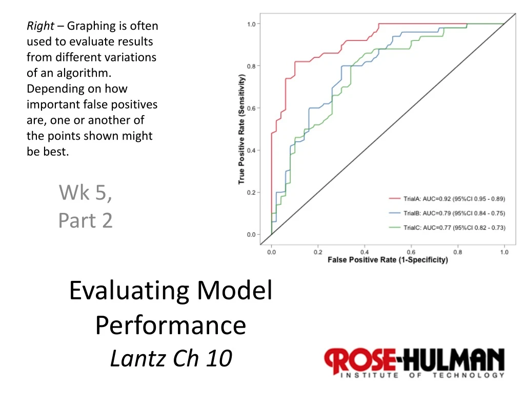
Right – Graphing is often used to evaluate results from different variations of an algorithm. Depending on how important false positives are, one or another of the points shown might be best. Evaluating Model Performance Lantz Ch 10 Wk 5, Part 2
A truckload of tricks • Lantz warns us that, in different domains, different ways are preferred, of deciding what results are “best”. • Includes many types of summary statistics, graphing for visual decisions, etc. • Our goal – you know where to look up and calculate any of these, if someone says, “Oh, and what’s the precision on that?” Etc.
Classifiers - Main types of data involved • Actual class values • Predicted class values • Estimated probability of the prediction • If two methods are equally accurate, but • One is more able to assess certainty, then • It is the “smarter” model.
Let’s look at ham vs spam again > sms_results <- read.csv("/Users/chenowet/Documents/Rstuff/sms_results.csv") > head(sms_results) actual_typepredict_typeprob_spam 1 ham ham 2.560231e-07 2 ham ham 1.309835e-04 3 ham ham 8.089713e-05 4 ham ham 1.396505e-04 5 spam spam 1.000000e+00 6 ham ham 3.504181e-03 This model is very confident of its choices!
How about when the model was wrong? > head(subset(sms_results, actual_type != predict_type)) actual_typepredict_typeprob_spam 53 spam ham 0.0006796225 59 spam ham 0.1333961018 73 spam ham 0.3582665350 76 spam ham 0.1224625535 81 spam ham 0.0224863219 184 spam ham 0.0320059616 Classifier knew it had a good chance of being wrong!
Confusion matrices tell the tale • We can judge based on what mistakes the algorithm made, • Knowing which ones we care most about.
E.g., predicting birth defects • Which kind of error is worse?
A common, global figure from these confusion matrices • An overall way to decide “accuracy” of an algorithm? Like, what percent is on the diagonal in the confusion matrix? “Error rate” is then 1 – accuracy.
So, for ham & spam… > CrossTable(sms_results$actual_type, sms_results$predict_type) Cell Contents |-------------------------| | N | | Chi-square contribution | | N / Row Total | | N / Col Total | | N / Table Total | |-------------------------| Total Observations in Table: 1390 | sms_results$predict_type sms_results$actual_type | ham | spam | Row Total | ------------------------|-----------|-----------|-----------| ham | 1202 | 5 | 1207 | | 16.565 | 128.248 | | | 0.996 | 0.004 | 0.868 | | 0.976 | 0.031 | | | 0.865 | 0.004 | | ------------------------|-----------|-----------|-----------| spam | 29 | 154 | 183 | | 109.256 | 845.876 | | | 0.158 | 0.842 | 0.132 | | 0.024 | 0.969 | | | 0.021 | 0.111 | | ------------------------|-----------|-----------|-----------| Column Total | 1231 | 159 | 1390 | | 0.886 | 0.114 | | ------------------------|-----------|-----------|-----------| Accuracy = (154 + 1202 )/ 1390 = 0.9755 Error rate = 0.0245
“Beyond accuracy” • The “kappa” statistic • Adjusts accuracy by accounting for a correct prediction by chance alone. • For our spam & ham, it’s 0.8867, vs 0.9775 • “Good agreement” = 0.60 to 0.80 • “Very good agreement” = 0.80 to 1.00 • Subjective categories
Sensitivity and specificity • Sensitivity = “True positive rate” and • Specificity = “True negative rate”
For ham and spam… > confusionMatrix(sms_results$predict_type, sms_results$actual_type, positive = "spam") Confusion Matrix and Statistics Reference Prediction ham spam ham 1202 29 spam 5 154 Accuracy : 0.9755 95% CI : (0.966, 0.983) No Information Rate : 0.8683 P-Value [Acc > NIR] : < 2.2e-16 Kappa : 0.8867 Mcnemar's Test P-Value : 7.998e-05 Sensitivity : 0.8415 Specificity : 0.9959 PosPred Value : 0.9686 NegPred Value : 0.9764 Prevalence : 0.1317 Detection Rate : 0.1108 Detection Prevalence : 0.1144 Balanced Accuracy : 0.9187 'Positive' Class : spam
Precision and recall • Also measures of the compromises made in classification. • How much the results are diluted by meaningless noise.
The F-measure • The “harmonic mean” of precision and recall. • Also called the “balanced F-score.” • There are also F1 and Fβ variants!
Visualizing • A chance to pick what you want based on how it looks vs other alternatives. • “ROC” curves – Receiver Operating Characteristic. • Detecting true positives vs avoiding false positives. Area under the ROC curve varies from 0.5 (no predictive value) to 1.0 (perfect).
For SMS data • “Pretty good ROC curve”:
Further tricks • Estimating future performance by calculating the “resubstitution error.” • Lantz doesn’t put much stock in these. • The “holdout method.” • Lantz has used this throughout. • Except it recommends holding out 25% – 50% of the data for testing, and he’s often used much less.
K-fold cross validation • Hold out 10% in different ways, 10 different times. • Then compare results of the 10 tests. • “Bootstrap sampling” – similar, but uses randomly selected training and test sets.