Download

1 / 25
250 likes | 285 Views
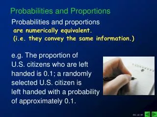
Explore the concepts of probabilities, sample spaces, permutations, and combinations. Learn how to interpret probability in various scenarios like coin tosses and free throws. Delve into the historical and theoretical aspects of probability theory.

E N D
15 Chances, Probabilities, and Odds 15.1 Random Experiments and Sample Spaces 15.2 Counting Outcomes in Sample Spaces 15.3 Permutations and Combinations 15.4 Probability Spaces 15.5 Equiprobable Spaces 15.6 Odds
What is Probability? If we toss a coin in the air, what is the probability that it will land heads up? Thisone is not a very profound question, and almost everybody agrees on the answer,although not necessarily for the same reason. The standard answer given is 1 outof 2, or 1/2. But why is the answer 1/2 and what does such an answer mean?
What is Probability? One common explanation given for the answer of 1/2 is that when we toss acoin, there are two possible outcomes (H and T), and since H represents one of the two possibilities, the probability of the outcome H must be 1 out of 2 or 1/2. This logic, while correct in the case of an honest coin, has a lot of holes in it.
Example 15.15 Who Is Shooting Those Free Throws? Imagine an NBA player in the act of shooting a free throw. Just like witha coin toss, there are two possible outcomes to the free-throw shot (success or failure), but it would be absurd to conclude that the probability ofmaking the free throw is therefore 1 out of 2, or 1/2. Here the two outcomes are not both equally likely, and their probabilities should reflectthat.
Example 15.15 Who Is Shooting Those Free Throws? The probability of a basketball player making a free throw very muchdepends on the abilities of the player doing the shooting–it makes a difference if it’s Steve Nash or Shaquille O’Neal. Nash is one of the best free-throw shooters in the history of the NBA, with a career average of 90%,while Shaq is a notoriously poor free-throw shooter (52% career average).
Empirical Interpretation of Probability Example 15.15 leads us to what is known as the empirical interpretationof the concept of probability. Under this interpretation when tossing an honest cointhe probability of Heads is 1/2 not because Heads is one out of two possible outcomes but because, if we were to toss the coin over and over–hundreds, possiblythousands, of times–in the long run about half of the tosses will turn out to beheads, a fact that has been confirmed by experiment many times.
Probability Theory The argument as to exactly how to interpret the statement “the probability ofX is such and such” goes back to the late 1600s, and it wasn’t until the 1930s that aformal theory for dealing with probabilities was developed by the Russian mathematician A.N. Kolmogorov (1903–1987). This theory has made probability one ofthe most useful and important concepts in modern mathematics. In the remainderof this chapter we will discuss some of the basic concepts of probability theory.
Events An event is any subset of the sample space. That is,an event is any set of individual outcomes. (This definition includes the possibility of an “event” that has nooutcomes as well as events consisting of a single outcome.) By definition, eventsare sets (subsets of the sample space), and we will deal with events using set notation as well as the basic rules of set theory.
Events A convenient way to think of an event is as a package in which outcomeswith some common characteristic are bundled together. Say you are rolling a pairof dice and hoping that on the next roll “you roll a 7”–that would make you temporarily rich. The best way to describe what really matters (to you) is by packaging together all the different ways to “roll a 7” as a single event E:
Events Sometimes an event consists of just one outcome. We will call such an event asimple event. In some sense simple events are the building blocks for all otherevents (more on that later). There is also the special case of the empty set { },corresponding to an event with no outcomes. Such an event can never happen,and thus we call it the impossible event.
Example 15.16 Coin-Tossing Event Let’s revisit the experiment of tossing a coin three times and recording the resultof each toss (Example 15.7). The sample space for this experiment isS = {HHH, HHT, HTH, HTT, THH, THT, TTH, TTT }.The set S has hundreds of subsets (256 to be exact), each of which represents a different event.Table 15-2 shows just a few of these events.
Example 15.17 The UnknownFree-Throw Shooter A player is going to shoot a free throw. We know nothing about his or her abilities–for all we know, the player could be Steve Nash, or Shaquille O’Neal, or Joe Schmoe,or you, or me.How can we describe the probability that he or she will make that freethrow? It seems that there is no way to answer this question, since we know nothing about the ability of the shooter. We could argue that the probability could bejust about any number between 0 and 1.
Example 15.17 The UnknownFree-Throw Shooter No problem–we make our unknownprobability a variable, say p. What can we say about the probability that our shooter misses the freethrow? A lot. Since there are only two possible outcomes in the sample space S = {s,f}the probability of success (s) and the probability of failure (f) mustcomplement each other–in other words, must add up to 1. This means that theprobability of missing the free throw must be 1 – p.
Example 15.17 The UnknownFree-Throw Shooter Table 15-3 is a summary of the line on a generic free-throw shooter.
Example 15.17 The UnknownFree-Throw Shooter Humbleas it may seem, Table 15-3 gives a complete model of free-throw shooting. Itworks when the free-throw shooter is Steve Nash (make it p = 0.90 ), ShaquilleO’Neal (make it p = 0.52), or the author of this book (make it p = 0.30). Eachone of the choices results in a different assignment of numbers to the outcomes inthe sample space.
Probability Assignment Example 15.17 illustrates the concept of a probability assignment. Aprobability assignment is a function that assigns to each event E a number between 0 and 1, which represents the probability of the event E and which we denote byPr(E). A probability assignment always assigns probability 0 to the impossibleevent[Pr({ }) = 0 and probability 1 to the whole sample space [Pr(S) = 1].
Probability Assignment With finite sample spaces a probability assignment is defined by assigningprobabilities to just the simple events in the sample space. Once we do this, wecan find the probability of any event by simply adding the probabilities of the individual outcomes that make up that event. There are only two requirements for avalid probability assignment: (1) All probabilities are numbers between 0 and 1,and (2) the sum of the probabilities of the simple events equals 1.
Example 15.18 Handicapping aTennis Tournament There are six players playing in a tennis tournament:A (Russian, female),B (Croatian, male), C (Australian, male), D (Swiss, male), E (American, female),and F (American, female).To handicap the winner of the tournament we need a probability assignmenton the sample space S = {A, B, C, D, E, F}.
Example 15.18 Handicapping aTennis Tournament With sporting events the probabilityassignment is subjective (it reflects an opinion), but professional odds-makers areusually very good at getting close to the right probabilities. For example, imaginethat a professional odds-maker comes up with the following probability assignment: Pr(A) = 0.08, Pr(B) = 0.16, Pr(C) = 0.20, Pr(D) = 0.25, Pr(E) = 0.16, Pr(F) = 0.15.
Example 15.18 Handicapping aTennis Tournament Once we have the probabilities of the simple events, the probabilities of allother events follow by addition. For example, the probability that an Americanwill win the tournament is given by Pr(E) + Pr(F) = 0.16 + 0.15 = 0.31.
Example 15.18 Handicapping aTennis Tournament Likewise, the probability that a male will win the tournament is given by Pr(B) + Pr(C) + Pr(D) = 0.16 + 0.20 + 0.25 = 0.61. The probability that anAmerican male will win the tournament is Pr({ }) = 0, since this one is an impossible event–there are no American males in the tournament!
Probability Space Once a specific probability assignment is made on a sample space, the combination of the sample space and the probability assignment is called a probabilityspace. The following is a summary of the key facts related to probability spaces.
ELEMENTS OF A PROBABILITY SPACE ■Sample space:S = {o1, o2,…,oN} ■Probability assignmentPr(o1),Pr(o2), …, Pr(oN) ■Events: These are all the subsets of S, including { } and S itself. The probability of an event is given by the sum of the probabilities of the individual outcomes that make up the event. [In particular, Pr({ }) = 0 and Pr(S) = 1.]