Download
1 / 62
620 likes | 636 Views
This study explores the CanCM4 climate model and its components, including the CanAM4 and CanOM4 models. It examines climate stability, biases in ocean surface temperature and salinity, and improvements in ENSO observations. The study also discusses decadal forecast initialization and alternative strategies for prediction, as well as climate projections to 2100. The CanCM4 model is used in various forecasting activities, including intra-seasonal, seasonal, and decadal forecasts.

E N D
Decadal Forecasts Using the CCCma Climate Model CanCM4 Bill Merryfield, Woo-Sung Lee, George Boer, Slava Kharin, John Scinocca and Greg Flato Canadian Centre for Climate Modelling and Analysis Environment Canada
CanCM4 model components • AGCM and OGCM new since AR4 • CanAM4 - T63/L35 - new shallow convection, radiation, aerosols… - includes “natural” volcanic & solar forcings • CanOM4 - 1.410.94 L40 (z~10m near surface) - GM stirring, KPP + tidal vertical mixing, anisotropic viscosity - solar penetrative heating according to climatological chlorophyll • Earth-system version CanESM2 used for long-term AR5 simulations
Mean=13.73C =0.12 C Mean=17.08Sv =0.78Sv CanCM4 climate stability 550 years of 1850 control run Global mean surface temperature Maximum Atlantic meridional overturning
CanCM4 surface ocean biases SST bias: Model - OISST 1982-2005 SST (C) SSS bias: Model – WOA/PHC 1982-2005 SSS (psu)
Model Improvement : ENSO Observations: HadISST 1970-99 CanAM3+CanOM3 CGCM3.1 (IPCC AR) CanAM3+CanOM4 CanAM4+CanOM4 CanCM4 CanCM3 Monthly SSTA standard deviation
AMO in CanCM4 control run Surface temperature regressed against AMO index NCEP Reanalysis 1948-2007 300 years of CanCM4 1850 control
AMO index time series Observed 1856-2008 300 years of CanCM4 1850 control
CCCma CMIP5 Decadal Prediction Experiments CORE EXPERIMENTS 3 different ocean initializations: Compare results choose one for application to remaining experiments additional predictions Initialized in ‘01, ’02, ’03 … ’09 hindcasts without volcanoes 10-year hindcast & prediction ensembles: initialized 1960, 1965, …, 2005 alternative initialization strategies prediction with 2010 Pinatubo-like eruption 30-year hindcast and prediction ensembles: initialized 1960, 1980 & 2005 increase ensemble sizes from O(3) to O(10) members
Climate projections to 2100+ CCCma contributions to international forecasting activities 45-60 days 12 months 10-30 years CanCM Intra- seasonal forecasts Seasonal forecasts Decadal forecasts Global Land-Atmosphere Coupling Experiment (GLACE-2) WCRP CHFP IPCC 5th Assessment (CMIP5) CanCM3 done CanCM4 in progress CanCM4 in progress CanCM3 done ~5000 years 7200 years US Clivar Intraseasonal Prediction Experiment CanCM4, to come
Initialization approach • Forecasts are launched from coupled “assimilation runs” • Assimilation runs constrain model atmosphere/SST/sea ice to be close to observational timeseries 1958-present • Different assimilation run for each ensemble member, starting from different initial conditions • Assimilation runs are preceded a multi-century spinup, subject to repeated 1960-1970 assimilation and ca.1958 radiative forcing - equilibrates upper ocean minimizes contribution of model drifts to forecast signal - provides suite of initial conditions for assimilation runs
Ocean initialization • 3 approaches tried core CMIP5 experiments performed for each - DHFP1A: ocean initial conditions from assimilation run surface forcing only - DHFP1B: full field ocean assimilation - DHFP1C: anomaly ocean assimilation
3D ocean T, S assimilation (GODAS after 1981, SODA before 1981) AGCM IRU assim (ERA) SST nudging (ERSST/OISST) Forecast Sea ice nudging (HadISST) + Anthropogenic & natural forcing 1 Oct 1 Nov 1 Dec 1 Jan 1 Feb 1 Sep multiple assimilation runs IC1 Forecast 2 Forecast 1 10-30 yearsd 10-30 years IC2 Spinup run … … … IC10 Forecast 10 12 mos Decadal forecast initialization
R R R R 0h 3h 6h 9h 12h 15h 18h DHFP Atmospheric Data Assimilation Incremental Reanalysis Update (IRU) assimilation: • run model freely for 3h (“forecast”) • difference with reanalysis “centered” increments xa • rewind, rerun for 6h, adding analysis increments as forcing to model equations: * To better reflect observational uncertainties in ensemble, “dial back” assimilation constant incremental nudging (CIN)
Pairwise standard deviations of air temperature vs height IRU Differences between reanalysis products CIN • Insert ¼ of increment • Truncate at T21
Benefits of IRU/CIN • accurate AGCM initialization essential for 1st month skill • ensemble generation • better land initialization • better ocean initialization/ background state for assimilation Due to “seeing” atmospheric forcing leading up to forecast
Impacts of AGCM assimilation on land initialization Correlation of assimilation run vs Guelph offline analysis SST nudging only SST nudging + AGCM assim Soil temperature (top layer) Soil moisture (top layer)
zonal wind stress thermocline depth zonal surface current sea surface temp Impacts of AGCM assimilation on ocean initialization Correlations vs obs in equatorial Pacific (5S 5N) SST nudging only SST nudging + IRU
CHFP2/DHFP1 Ocean data assimilation • T assimilation - procedure of Tang et al. JGR 2004 - off-line variational assimilation of 3D gridded analyses • S assimilation - procedure of Troccoli et al. MWR 2002 - preservation of T-S relationship: prevents spurious convection, etc. Nino3.4 anomaly correlation: from 1 Sep 1980-2001 (6 ensemble members) (Old model version: CanAM3 + CanOM3.6
-1.2 -1.0 -.8 -.6 -.4 -.2 -1.2 -1.0 -.8 -.6 -.4 -.2 0 0 .2 .4 .6 .8 1.0 1.2 .2 .4 .6 .8 1.0 1.2 Full field vs anomaly ocean assimilation Temperature increments in equatorial Pacific (upper 1000m) for 1 Jan 1981 DHFP1B Full field assim DHFP1C Anomaly assim
Properties of Assimilation Runs & Forecast Initial Conditions
rms T (C) Assimilation runs: Ensemble spread rms potential temperature difference between two members of assimilation run ensemble 56 m depth 510 m depth
Assimilation runs: Ensemble spread Potential temperature difference at 510m depth between two members of assimilation run ensemble 1995-2003 Temperature (C)
Ocean initial conditions: Ensemble spread Time series of maximum Atlantic meridional overturning at 26N in assimilation run ensemble
DHFP assimilation run 1990-94 CanCM4 control North Atlantic mixed layer depth (March) Obs (Levitus 94) DHFP assimilation run 1975-79
Comparison with other analyses max overturning Avg of CCCma assimilation runs (ERA forced) Reconstructed from NCEP GECCO Reconstructed from ERA max overturning 48N ECMWF ocean analysis Grist et al.JClim 2009
Comparison with other analyses max overturning Avg of CCCma assimilation runs (ERA forced) Reconstructed from NCEP GECCO Reconstructed from ERA max overturning 48N ECMWF ocean analysis Grist et al.JClim 2009
Comparison with other analyses 3 2 1 max overturning 26N 0 Avg of CCCma assimilation runs (ERA forced) -1 -2 Reconstructed from obs SST + HadCM3* Analog forecasts max overturning 30N Knight et al.GRL 2005 *based on running decadal means
1.0 0.6 0.4 0.5 0.2 0 Correlation Correlation 0 -0.5 -0.2 -1.0 -0.4 -20 -20 -10 -10 0 0 10 10 20 20 Lag of overturning lag vs AMO (years) Lag of overturning lag vs AMO (years) Overturning vs AMO relationship in model & obs Lag correlation of max Atlantic meridional overturning vs AMO index Based on running 11-year means Overturning and AMO from 300 years of CanCM4 1850 control Overturning from assimilation run; AMO from obs 1958-2008 Similarity of phasing vs control run of assimilation run overturning + observed AMO suggests that assimilation run overturning could be ~ realistic
Decadal forecast results to 2015 DHFP1A: Surface forcing only
Decadal forecast results to 2015 DHFP1A: Surface forcing only 1 to 10-year means -
Decadal forecast results to 2015 DHFP1A: Surface forcing only Anomaly correlation skill -
Impact of ocean initialization DHFP1B: Full field assimilation DHFP1A: Surface forcing only DHFP1C: Anomaly assimilation CanESM2 (5 1850-2005 historical runs)
Impact of ocean initialization 1 to 10-year means DHFP1B: Full field assimilation DHFP1A: Surface forcing only DHFP1C: Anomaly assimilation CanESM2 (5 1850-2005 historical runs)
Decadal forecast results to 2015 DHFP1A: Surface forcing only
Correlation of forecast and analysis MOC anomalies DHFP1A: Surface forcing only
Impact of ocean initialization DHFP1B: Full field assimilation DHFP1A: Surface forcing only DHFP1C: Anomaly assimilation CanESM2 (5 1850-2005 historical runs)
North Atlantic Overturning Control run 10 year mean vs assimilation & forecast 1981 means (1st year of forecast) Control run Assimilation run DHFP1B: Full field assim DHFP1A: Surface forcing only
Impact of ocean initialization SEP SEA ICE AREA NH (M2) DHFP1B: Full field assimilation DHFP1A: Surface forcing only DHFP1C: Anomaly assimilation CanESM2 (5 1850-2005 historical runs)
Anomaly correlation skill Mean for individual year forecasts *poor pre-1979 verification data *includes poor pre-satellite era verifications which probably should be excluded **through 2005
Anomaly correlation skill Mean for 1-10 year mean forecasts *poor pre-1979 verification data *includes poor pre-satellite era verifications which probably should be excluded **through 2005
Persisted trend forecast Decadal trend Persisted trend HadCRUT3 global mean surface temperature anomaly
RMSE RMSE DHFP1A DHFP vs persisted trend forecast RMSE mean(DHFP1A rmse) = 0.123340 mean(DHFP1B rmse) = 0.132509 mean(DHFP1C rmse) = 0.124645 DHFP1B mean(persisitence rmse) = 0.139910 mean(persisited trend rmse)= 0.114405 DHFP1C 1 10 Year of forecast
Correlation skill map DHFP1A: Surface forcing only DHFP1B: Full field assim First 1/2 year First year First 2 years First 4 years
Potential correlation* Forecast correlation 1/12 1/6 1/4 1/2 1 2 3 4 6 8 10 Averaging period (years) DHFP1A: surface forcing only DHFP1B: full field assim *from analysis of variance
Decadal predictability: surface temp Potentially predictable variance fraction, from Boer (Clim Dyn 2010) Internally generated (control climate) Next decade, including forced change based on CMIP3 models
Correlation skill Next decade predictability