Download

1 / 35
360 likes | 490 Views
This document delves into the theory behind Min-Plus linear systems and their application in estimating available bandwidth within network systems. It covers the fundamentals of linear time-invariant systems, the concept of impulse response, and the unique min-plus convolution method. Various scenarios are explored, including the analysis of arrival and departure functions, as well as network probing techniques. The text outlines how to measure packet transfers and utilize service curves to estimate network capabilities, providing a comprehensive understanding of the interplay between mathematical modeling and practical network performance.

E N D
Min-Plus Linear Systems TheoryandBandwidth Estimation TexPoint fonts used in EMF. Read the TexPoint manual before you delete this box.:
Linear: Time invariant: (Classical) System Theory Linear Time Invariant (LTI) Systems
Linear Systems Theory Consider an input signal: .. and its output at a system: Note:
Linear Systems Theory • Consider an arbitrary function • Approximate by Now we let
Linear Systems Theory • The result of Impulse Response “convolution”
If input is Dirac impulse, output is the system response • Output can be calculated from input and system response: “convolution” (Classical) System Theory Linear Time Invariant (LTI) Systems
Min-Plus Linear System min-plus Linear: Time invariant:
Min-Plus Linear System Consider arrival function: .. and departure function: Note:
Min-Plus Linear System • Consider an arbitrary function • Approximate by Now we let
Min-Plus Linear System • The result of “min-plus convolution” Service Curve
Min-Plus Linear Systems • If input is burst function , output is the service curve
Min-Plus Linear Systems • Departures can be calculated from arrivals and service curve: “min-plus convolution”
Back to (Classical) Systems Time Shift System eigenfunction eigenvalue eigenfunction • Now: • Eigenfunctions of time-shift systems are also eigenfunctions of any linear time-invariant system
Back to (Classical) Systems eigenvalue • Solving: • Gives: Fourier Transform
Now Min-Plus Systems again Time Shift System eigenfunction eigenvalue eigenfunction • Now: • Eigenfunctions of time-shift systems are also eigenfunctions of any linear time-invariant system
Back to (Classical) Systems eigenvalue • Solving: • Gives: Legendre Transform
System Theory for Networks • Networks can be viewed as linear systems in a different algebra: • Addition (+) Minimum (inf) • Multiplication (·) Addition (+) • Network service is described by a service curve Min-Plus Algebra
Transforms • Classical LTI systems Frequency domain Time domain Fourier transform • Min-plus linear systems Rate domain Time domain Legendre transform Properties: (1) . If is convex: (2) If convex, then (3) Legendre transforms are always convex
Available Bandwidth • Available bandwidth is the unused capacity along a path • Available bandwidth of a link: • Available bandwidth of a path: • Goal: Use end-to-end probing to estimate available bandwidth Edited slide from: V. Ribeiro, Rice. U, 2003
Probing a network with packet trains • A network probe consists of a sequence of packets (packet train) • The packet train is from a source to a sink • For each packet, a measurement is taken when the packet is sent by the source (arrival time), and when the packet arrives at the sink (departure time) • So: rate at which the packet trains are sent is crucial: • Rate too high probes preempt existing traffic • Rate too low probes only measure the input rate source sink Edited slide from: V. Ribeiro, Rice. U, 2003
Rate Scanning Probing Method • Each packet trains is sent at a fixed rate r (in bits per second). This is done by: • All packets in the train have the same size • Packets of packet train are sent with same distance • If size of packets is L, transmission time of a packet is T, and distance between packets is D, the rate is: r = L/(T+D) • Rate Scanning: Source sends multiple packet trains, each with a different rate r Packet train: D D D
Min-Plus Linear Systems min-plus Linear: Time invariant: • Departures can be calculated from arrivals and service curve: • If input is burst function , output is the service curve “min-plus convolution”
One more thing … • Many networks are not min-plus linear • i.e., for some t: • … but can be described by a lower service curve • such that for all t: • Having a lower service curve is often enough, since it provides a lower bound on the service !!
View the network as a min-plus system that is either linear or nonlinear Bandwidth estimation scheme: 1. Timestamp probes Ap(t) - Send probes Dp(t) - Receive probes 2. Use probes to find a that satisfies for all (A,D). 3. is the estimate of the available bandwidth. Bandwidth estimation in the network calculus
View the network as a min-plus system that is either linear or nonlinear Bandwidth estimation scheme: 1. Timestamp probes Ap(t) - Send probes Dp(t) - Receive probes 2. Use probes to find a that satisfies for all (A,D). 3. the goal is to select as large as possible. Bandwidth estimation in the network calculus
Bandwidth estimation in a min-plus linear network • If network is min-plus linear, we get • If we set , then • So: We get an exact solution when the probe consist of a burst (of infinite size and sent with an infinite rate) • However: • An infinite-sized instantaneous burst cannot be realized in practice(It also creates congestion in the network)
Rate Scanning (1): Theory • Backlog: • Max. backlog: • If , we can write this as: • Inverse transform: If S is convex we have
Rate Scanning (2): Algorithm Step 1: Transmit a packet train at rate , compute compute Step 2: If estimate of has improved, increase and go to Step 1. • This method is very close to Pathload !
Non-Linear Systems • When we exploit we assume a min-plus linear system • In non-linear networks, we can only find a lower service curve that satisfies • We view networks as system that are always linear when the network load is low, and that become non-linear when the network load exceeds a threshold. • Note: In rate scanning, by increasing the probing rate, we eventually exceed the threshold at which the network becomes non-linear • QUESTION: How to determine the critical rate at which network becomes non-linear
Detecting Non-linearity Backlog convexity criterion • Suppose that we probe at constant rates • Legendre transform is always convex • In a linear system, the max. backlog is the Legendre transform of the service curve: • If we find that for some rate r we know that system is not linear
Emulab is a network testbed at U. Utah can allocate PCs and build a network controlled rates and latencies Some Questions: How well does our theory translate to real networks? Does representing available bandwidth by a function (as opposed to a number) have advantages? How robust are the methods to changes of the traffic distribution? EmuLab Measurements
Dumbbell Network • UDP packets with 1480 bytes (probes) and 800 bytes (cross) • Cross traffic: 25 Mbps
Constant Bit Rate (CBR) Cross Traffic • Cross traffic is sent at a constant rate (=CBR) • The “reference service curve” (red) shows the ideal results. The “service curve estimates” shows the results of the rate scanning method • Figure shows 100 repeated estimates of the service curve Rate Scanning
Rate Scanning: Different Cross Traffic • Exponential: random interarrivals, low variance • Pareto: random interarrivals, very high variance Pareto Exponential
Dirac impulse • The Diract delta function, often referred to as the unit impulse function, can usually be informally thought of as a function δ(x) that has the value of infinity for x = 0, the value zero elsewhere. The integral from minus infinity to plus infinity is 1. From: Wikipedia