Download
1 / 53
530 likes | 669 Views
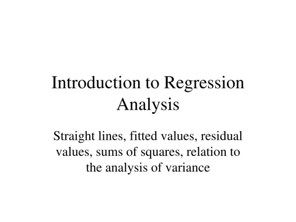
Introduction to Regression Lecture 2.2. Review of Lecture 2.1 Homework Multiple regression Job times case study Job times continued residual analysis model fitting and testing Model fitting and testing procedure t-tests Analysis of Variance. Update: Accessing data files.

E N D
Introduction to RegressionLecture 2.2 • Review of Lecture 2.1 • Homework • Multiple regression • Job times case study • Job times continued • residual analysis • model fitting and testing • Model fitting and testing procedure • t-tests • Analysis of Variance Diploma in Statistics Introduction to Regression
Update: Accessing data files • Access the data in mstuart's get folder: • in ISS Public Access labs, click Start, then Network Shortcuts, open Get • on your own computer with TCD network access, navigate to Ntserver-usr / get • once in get, type ms, open mstuart, Diploma Reg, Excel Data, or • Access the data on the Diploma web page at https://www.scss.tcd.ie:453/courses/dipstats/Local/ST7002_0809.php • Open the relevant Excel file and copy the data Diploma in Statistics Introduction to Regression
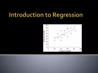
Homework 2.1.1 The shelf life of packaged foods depends on many factors. Dry cereal (such as corn flakes) is considered to be a moisture-sensitive product, with the shelf life determined primarily by moisture. In a study of the shelf life of one brand of cereal, packets of cereal were stored in controlled conditions (23°C and 50% relative humidity) for a range of times, and moisture content was measured. The results were as follows. Draw a scatter diagram. Comment. What action is suggested? Why? Diploma in Statistics Introduction to Regression
Draw a scatter diagram. Comment. What action is suggested? Why? 2 exceptional cases; delete and investigate Diploma in Statistics Introduction to Regression
Following appropriate action, the following regression was computed. The regression equation is Moisture = 2.86 + 0.0417 Storage Predictor Coef SE Coef T P Constant 2.86122 0.02488 115.01 0.000 Storage 0.041660 0.001177 35.40 0.000 S = 0.0493475 Calculate a 95% confidence interval for the daily change in moisture content; show details. Diploma in Statistics Introduction to Regression
Was the action you suggested on studying the scatter diagram in part (a) justified? Explain. Predict the moisture content of a packet of cereal stored under these conditions for 5 weeks; calculate a prediction interval. What would be the effect on your interval of not taking the action you suggested on studying the scatter diagram? Why? Taste tests indicate that this brand of cereal is unacceptably soggy when the moisture content exceeds 4. Based on your prediction interval, do you think that a box of cereal that has been on the shelf for 5 weeks will be acceptable? Explain. What about 4 weeks? 3 weeks? What is acceptable? Diploma in Statistics Introduction to Regression
Introduction to RegressionLecture 2.2 • Review of Lecture 2.1 • Homework • Multiple regression • Job times case study • Job times continued • residual analysis • model fitting and testing • Model fitting and testing procedure • t-tests • Analysis of Variance Diploma in Statistics Introduction to Regression
Example 5A production prediction problem Erie Metal Products: The problem Metal products fabrication: customers order varying quantities of products of varying complexity; customers demand accurate and precise order delivery times. Diploma in Statistics Introduction to Regression
Erie Metal Products: The data Diploma in Statistics Introduction to Regression
The multiple linear regression model Jobtime = a + bUnits× Units + bOps× Ops + bT_Ops× T_Ops + bRushed× Rushed + e Diploma in Statistics Introduction to Regression
Model parameters The regression coefficients: a, bUnits, bOps, bT_Ops, bRushed The "uncertainty" parameter: s= standard deviation of e Diploma in Statistics Introduction to Regression
Regression of Jobtime on other variables Predictor Coef SE Coef T P Constant 77.24 44.76 1.73 0.105 Units -0.1507 0.1121 -1.34 0.199 Ops 7.152 4.305 1.66 0.117 T_Ops 0.11460 0.01322 8.67 0.000 Rushed -24.94 19.11 -1.31 0.211 S = 37.4612 Diploma in Statistics Introduction to Regression
Homework Predict job times for small (U=100, O=5), medium (U=300, O=10) and large (U=500, O=15) jobs, both normal and rushed. Present the results in tabular form. Diploma in Statistics Introduction to Regression
Homework Solution Diploma in Statistics Introduction to Regression
Are these predictions useful? What is S? What is 2S? When will my order arrive? NEXT Diagnostics; analysis of residuals Diploma in Statistics Introduction to Regression
Introduction to RegressionLecture 2.2 • Review of Lecture 2.1 • Homework • Multiple regression • Job times case study • Job times continued • residual analysis • model fitting and testing • Model fitting and testing procedure • t-tests • Analysis of Variance Diploma in Statistics Introduction to Regression
Checking model fit Assumptions: explanatory variables are adequate error term (): variation is Normal variation is stable Check via residuals Response = Fit + Residual Diploma in Statistics Introduction to Regression
Regression diagnostics • The diagnostic plot, 'deleted' residuals vs fitted values • checking for homogeneity of error • The Normal residual plot, • checking the Normal model Diploma in Statistics Introduction to Regression
Residuals Job 9, a rushed job with 21 units and 9 operations per unit, took 260 hours to complete. Prediction Jobtime = 77 – 0.15 × 21 + 7.1 × 9 + 0.11 × 189 – 25 = 135, Residual = 260– 135 = 125 Diploma in Statistics Introduction to Regression
Deleted residuals Job 9, a rushed job with 21 units and 9 operations per unit, took 260 hours to complete. Deleted prediction, regression with case 9 deleted: Jobtime = 42 – 0.08× 21 + 10× 9 + 0.11× 189 - 38 = 113, Deleted Residual = 260– 113 = 147 Standardised deleted residual ≈ DR / s = 147 / 14 = 10.5 Diploma in Statistics Introduction to Regression
Deleted residuals • Residual • observed – fitted • Standardised Residual • using an estimate of s based on current data • Standardised Deleted Residual • calculated from data with suspect case deleted • s estimated from data with suspect case deleted Diploma in Statistics Introduction to Regression
The Diagnostic Plot Diploma in Statistics Introduction to Regression
Scatterplot of artificial datawith a highly exceptional case NB: exceptionally large Y value corresponds to small X value Diploma in Statistics Introduction to Regression
Scatter plot and diagnostic plotfor artificial data Diploma in Statistics Introduction to Regression
Normal plot of residuals Diploma in Statistics Introduction to Regression
Statistical AnalysisSection 8.4Iterating the analysis • Revising the fit • revised prediction formula • revised diagnostics • A further iteration Diploma in Statistics Introduction to Regression
Revised fit, case 9 deleted The regression equation is Jobtime = 41.7 – 0.0835 Units + 10.0 Ops + 0.110 T_Ops – 38.2 Rushed 19 cases used, 1 cases contain missing values Predictor Coef SE Coef T P Constant 41.72 16.87 2.47 0.027 Units -0.08349 0.04186 -1.99 0.066 Ops 10.022 1.612 6.22 0.000 T_Ops 0.110016 0.004891 22.49 0.000 Rushed -38.217 7.166 -5.33 0.000 S = 13.7952 Diploma in Statistics Introduction to Regression
Revised fit Exercise Predict job times for small (U=100, O=5), medium (U=300, O=10) and large (U=500, O=15) jobs, normal and rushed. Diploma in Statistics Introduction to Regression
Revised predictions Diploma in Statistics Introduction to Regression
Recall scatter plot for artificial data Diploma in Statistics Introduction to Regression
Revised diagnostics, case 9 deleted Diploma in Statistics Introduction to Regression
Revised fit, cases 9, 11, 16 deleted The regression equation is Jobtime = 44.2 – 0.0693 Units + 9.83 Ops + 0.108 T_Ops – 38.0 Rushed 17 cases used, 3 cases contain missing values Predictor Coef SE Coef T P Constant 44.216 9.080 4.87 0.000 Units –0.06931 0.02853 –2.43 0.032 Ops 9.8286 0.8873 11.08 0.000 T_Ops 0.107795 0.004114 26.20 0.000 Rushed –37.960 3.857 –9.84 0.000 S = 7.41272 Diploma in Statistics Introduction to Regression
Revised diagnostics, cases 9, 11, 16 deleted Diploma in Statistics Introduction to Regression
Coefficient estimates from three fits Diploma in Statistics Introduction to Regression
Homework 2.2.1 Extend table of predictions of small medium and large jobs to include predictions based on the final fit. Compare and contrast. Diploma in Statistics Introduction to Regression
Introduction to RegressionLecture 2.2 • Review of Lecture 2.1 • Homework • Multiple regression • Job times case study • Job times continued • residual analysis • model fitting and testing • Model fitting and testing procedure • t-tests • Analysis of Variance Diploma in Statistics Introduction to Regression
The model fitting and testing procedure • Step 1: Initial data analysis: • Step 2: Least squares fit and interpretation: • Step 3: Diagnostic analysis of residuals: • Step 4: Iterate fit and check: Diploma in Statistics Introduction to Regression
Step 1: Initial data analysis • standard single variable summaries • to determine extent of variation • possible exceptional values; • scatter plot matrix • to view pair wise relationships between the response and the explanatory variables and • to view pair wise relationships between the explanatory variables themselves. Diploma in Statistics Introduction to Regression
Step 2: Least squares fit and interpretation • calculate the best fitting regression coefficients • check meaningfulness and statistical significance; • calculate s • check its usefulness for prediction • its usefulness relative to alternative estimates of standard deviation. Diploma in Statistics Introduction to Regression
Step 3: Diagnostic analysis of residuals • diagnostic plot • check for exceptional residuals or patterns of residuals, • possible explanations in terms of the fitted values; • Normal plot • check for exceptional residuals or non-linear patterns in the residuals Diploma in Statistics Introduction to Regression
Step 4: Iterate fit and check • determine cases for deletion • repeat steps 2 and 3 until checks are passed. Diploma in Statistics Introduction to Regression
Homework 2.2.2 You have been asked to comment, as a statistical consultant, on a prediction formula for forecasting job completion times prepared by a former employee. The formula is, effectively, the one derived from the first fit discussed above. Write a report for management. Your report should refer to (i) the practical usefulness of the employee's prediction formula, from a customer's perspective, (ii) the significance of the exceptional cases from the customer's and management's perspectives, and (iii) your recommended formula, with its relative advantages. Diploma in Statistics Introduction to Regression
Introduction to RegressionLecture 2.2 • Review of Lecture 2.1 • Homework • Multiple regression • Job times case study • Job times continued • residual analysis • model fitting and testing • Model fitting and testing procedure • t-tests • Analysis of Variance Diploma in Statistics Introduction to Regression
t-tests First fit The regression equation is Jobtime = 77.2 – 0.151 Units + 7.15 Ops + 0.115 T_Ops – 24.9 Rushed Predictor Coef SE Coef T P Constant 77.24 44.76 1.73 0.105 Units –0.1507 0.1121 –1.34 0.199 Ops 7.152 4.305 1.66 0.117 T_Ops 0.11460 0.01322 8.67 0.000 Rushed –24.94 19.11 –1.31 0.211 S = 37.4612 Diploma in Statistics Introduction to Regression
Revised fit, case 9 deleted The regression equation is Jobtime = 41.7 – 0.0835 Units + 10.0 Ops + 0.110 T_Ops – 38.2 Rushed 19 cases used, 1 cases contain missing values Predictor Coef SE Coef T P Constant 41.72 16.87 2.47 0.027 Units -0.08349 0.04186 -1.99 0.066 Ops 10.022 1.612 6.22 0.000 T_Ops 0.110016 0.004891 22.49 0.000 Rushed -38.217 7.166 -5.33 0.000 S = 13.7952 Diploma in Statistics Introduction to Regression
Revised fit, cases 9, 11, 16 deleted The regression equation is Jobtime = 44.2 – 0.0693 Units + 9.83 Ops + 0.108 T_Ops – 38.0 Rushed 17 cases used, 3 cases contain missing values Predictor Coef SE Coef T P Constant 44.216 9.080 4.87 0.000 Units –0.06931 0.02853 –2.43 0.032 Ops 9.8286 0.8873 11.08 0.000 T_Ops 0.107795 0.004114 26.20 0.000 Rushed –37.960 3.857 –9.84 0.000 S = 7.41272 Diploma in Statistics Introduction to Regression
Homework 2.2.3 Make a table of the t values and corresponding s values for the three regressions Compare, contrast and explain. Diploma in Statistics Introduction to Regression
Introduction to RegressionLecture 2.2 • Review of Lecture 2.1 • Homework • Multiple regression • Job times case study • Job times continued • residual analysis • model fitting and testing • Model fitting and testing procedure • t-tests • Analysis of Variance Diploma in Statistics Introduction to Regression
Analysis of Variance S = 7.41272 R-Sq = 99.8% R-Sq(adj) = 99.7% Analysis of Variance Source DF SS MS F P Regression 4 299165 74791 1361.12 0.000 Residual Error 12 659 55 Total 16 299824 Residual Mean Square = s2: check! Diploma in Statistics Introduction to Regression
Analysis of Variance Regression Sum of Squares measures explained variation Residual Sum of Squares measures unexplained (chance) variation Total Variation = Explained + Unexplained Check it! Diploma in Statistics Introduction to Regression