Scaling Three-dimensional Fourier Transforms
290 likes | 473 Views
Scaling Three-dimensional Fourier Transforms . Dmitry Pekurovsky dmitry@sdsc.edu San Diego Supercomputer Center. Fast Fourier Transform (FFT). F(k) = S x f(x) exp(-i2 p kx/N) A well-known, efficient, commonly used algorithm 1D FFT used in MANY science fields

Scaling Three-dimensional Fourier Transforms
E N D
Presentation Transcript
Scaling Three-dimensional Fourier Transforms Dmitry Pekurovsky dmitry@sdsc.edu San Diego Supercomputer Center
Fast Fourier Transform (FFT) F(k) = Sx f(x) exp(-i2pkx/N) • A well-known, efficient, commonly used algorithm • 1D FFT used in MANY science fields • Implemented in almost every scientific library (e.g. ESSL, NAG, MKL) • Open-source software • FFTW • 3D FFT is fairly commonly used too • Turbulence simulations • Reverse tomography • Cosmology • Ocean science • Molecular Dynamics
1D FFT • Cooley-Tukey algorithm (1965) • Divide-and-conquer algorithm • Break up FT size N into N1 N2 – even and odd indices • Keep going until reach size 2 • Complexity O(N logN)
3D Fourier Transform in parallel: strategy • Problem: grid N x N x N distributed over Np processors • Would like to do 1D FFT in each of the three dimensions • Not all data in a given dimension may be local to any processor Strategy • Direct approach: parallel version of 1D FFT – many processors take part, sending data when needed • Transpose approach • Rearrange data in advance to make it always local for the dimension to be transformed. • All processors call regular 1D FFT Lots of communication in both cases, but transpose approach is better: need to communicate only once, right before the local 1D FFT.
Typical parallel 3D FFT up to now • Transpose strategy, 1D decomposition • Each CPU has several planes (slabs) • Local geometry: N x N x L, where L=N/P • Transform in 2 dimensions local to the planes first • Use an established library for 1D FFT, e.g. ESSL, FFTW • Transpose data to localize third dimension • Local geometry: N x L x N • Complete transform by operating along third dimension • Most everyone has been using this approach. Examples: • PESSL • NAS Parallel Benchmarks
1D decomposition scaling • Communication: 1 call to MPI_Alltoall or equivalent all-to-all exchange. • Demanding operation. Performance depends on interconnect bisection bandwidth. • Cut the network in two. Count the links cut. • This parameter depends on bandwidth of each link, and also network topology (e.g. fat-tree for Datastar, 3D torus for Blue Gene) • Can scale OK (depending on interconnect), but only up to a point: P <= N • For 4096^3 grid, no more than 4096 processors. But we need a lot more even to fit in memory. • => A new approach is needed
2D decomposition y x z
2D decomposition • 2D decomposition: processors form a square grid P1 x P2 • Columns (pencils) instead of slabs • Local geometry: • Stage 1: N x K x M • Stage 2: K x N x M • Stage 3: K x M x N • K = N/P1, M=N/P2 • At each stage, transform along the local dimension (N) • Software scaling limit removed! Now the limit is P <= N2
MPI Implementation • Setup stage: create two subcommunicators, for rows and columns: integer periodic(2),remain_dims(2),cartid(2),dims(2),comm_cart,comm_row,comm_col periodic(1) = .false. periodic(2) = .false. call MPI_Cart_create(MPI_COMM_WORLD,2,dims,periodic,.false.,comm_cart,ierr) call MPI_Cart_coords(comm_cart,taskid,2,cartid,ierr) remain_dims(1) = .true. remain_dims(2) = .false. call MPI_Cart_sub(comm_cart,remain_dims,comm_row,ierr) remain_dims(1) = .false. remain_dims(2) = .true. call MPI_Cart_sub(comm_cart,remain_dims,comm_col,ierr)
MPI implementation • First transpose call MPI_Alltoall(sendbuf,Ncount,MPI_DOUBLE, recvbuf,Ncount,MPI_DOUBLE,comm_row,ierr) • Second transpose call MPI_Alltoall(sendbuf,Ncount,MPI_DOUBLE, recvbuf,Ncount,MPI_DOUBLE,comm_col,ierr)
What about overlapping communication with computation? • In general it’s a good idea • There isn’t a non-blocking version of MPI_Alltoall is the MPI standard today • Need to write your own, based on MPI_Isend, MPI_Irecv, MPI_Wait • Performance advantage will depend on platform • Blue Gene/L is not equipped with capabilities for overlap. CPUs are busy transmitting data. • Next generation of machines likely to have RDMA capabilities (Remote Direct Memory Access)
Some rules of thumb • Aggregate data and call MPI as few times as possible • Derived datatypes are convenient but are often a disadvantage in performance • Try to minimize the number of memory copies – do in-place operations if feasible • If possible, try to use array stride 1 • When calling 1D FFT give it many transforms to do at a time
Implementation and Performance Each processor doing a (large) number of 1D FFT • Memory access stride is a crucial parameter • FFT in X, stride 1: 28% peak on Datastar • Transpose in X & Y • FFT in Y, stride Nx/P1: 25% peak on Datastar • Transpose in Y & Z • FFT in Z, stride (NxNy)/P: 10% peak on Datastar • Alternative is to rearrange in memory space so that stride is 1. Involves an extra memory load. • ESSL is about 3 times faster than FFTW. • Always use native high-performance library if available
Implementation in a code • Originally implemented in DNS (Direct Numerical Simulations) turbulence code • Prof. P.K.Yeung, Georgia Tech • Part of SAC project (Strategic Applications Collaboration, http://www.sdsc.edu/us/sac) • Algorithm: straight 2nd order Runge-Kutta in time, pseudospectal in space. • 3D FFT is ~70% of the computation, and ~95% communication • Researchers interested in grid sizes 40963 and beyond • (Earth Simulator apparently the only machine to handle this size to date, in 2002!). • More than 4096 processors are likely needed due to memory and compute power. • Face the 1D decomposition software limitation • Ran 40963 test problem with 2D decomposition on Blue Gene at IBM T.J.Watson lab, up to 32k CPUs.
Performance of DNS (2D) on IBM Blue Gene VN: Two processors per node CO: One processor per node
Communication and performance: 2D vs. 1D • 1D: 1 All-to-all exchange over P tasks • 2D: 2 All-to-all exchanges in groups: • P2 groups of P1 tasks each • P1 groups of P2 tasks each • Which is better? • Message size decreases if the exchange group size increases • Some links are unused in each of the 2 transposes, and data volume is the same as in 1D case • 1D decomposition ends up winning • But again: 1D is only good up to P = N
Choosing P1 and P2 • P1 x P2 = P • If P <= N, choose P1 = 1 (1D decomposition is better) • If P >N, in most cases it’s best to choose smallest P1 (= P/N) • Better communication pattern • In some cases, better cache use: arrays leading dimension is N/ P1 which is a problem if it gets to be less than the cache line.
P3DFFT • Open source library for efficient, highly scalable 3D FFT on parallel platforms • Built on top of an optimized 1D FFT library • Currently ESSL or FFTW • In the future, more libraries • Uses 2D decomposition, with option for 1D. • Available at http://www.sdsc.edu/us/resources/p3dfft.php • Current status: basic version available, more work is under way.
P3DFFT: more features • Implements real-to-complex (R2C) and complex-to-real (C2R) 3D transforms • Written in Fortran 90 with MPI • Implemented as F90 module • Single or double precision • Arbitrary dimensions • Handles many uneven cases (Ni does not have to be a factor of Pj) • Assume Ni >= Pj • Can do either in-place transform or otherwise • In which case the input and output arrays should not overlap • Memory requirements: input and output arrays + 1 buffer
P3DFFT: Storage • R2C transform input: • Global: (Nx,Ny,Nz) real array • Local: (Nx,Ny/P1,Nz/P2) real array • R2C output: • Global: (Nx/2+1,Ny,Nz) complex array • Conjugate symmetry: F(N-i) = F*(i) • F(N/2+1) through F(N-1) are redundant • F(0) and F(N/2) are real • Total N/2+1 complex storage units • Local: ((Nx+2)/(2P1),Ny/P2,Nz) complex • C2R: input and output interchanged from R2C
Building P3DFFT • Subdirectory build/ • Edit makefile for your architecture • Specify -DSINGLE_PREC or -DDOUBLE_PREC • Default is single precision • Specify -DESSL or -DFFTW • Choose P3DFFT_ROOT • Type ‘make’ – will compile and install the library in P3DFFT_ROOT directory • On SDSC platforms, it is already installed in /usr/local/apps/p3dfft • Subdirectory sample/ • Contains sample programs • For manual see README file in upper level directory
Using P3DFFT • ‘use p3dfft’ • Defines mytype – 4 or 8 byte reals • Initialization: p3dfft_setup(proc_dims,nx,ny,nz) • procs_dims(2) – two integers, P1 and P2 • For 1D decomposition, set P1 = 1 • Sets up the square 2D grid of MPI communicators in rows and columns • Initializes local array dimensions • Local dimensions: get_dims(istart,iend,isize,Q) • istart(3),iend(3),isize(3) – X,Y,Z bounds for local domains • Set Q=1 for R2C input, Q=2 for R2C output
Using P3DFFT (2) • Now allocate your arrays • When ready to call transform: p3dfft_ftran_r2c(IN,OUT) – Forward transform • exp(-ikx/N) p3dfft_btran_c2r(IN,OUT) – Backward (inverse) transform • exp(ikx/N)
Future work • Include more array distribution schemes • Expand options for memory ordering • Include more transform types • Derivatives • Complex-to-complex • C interface • Convenience functions • Break down in stages • Expand choice of 1D FFT libraries • Questions? Comments? dmitry@sdsc.edu
P3DFFT and Petascale • This algorithm is applicable to a large number of problems, in particular DNS turbulence • One of the three model problems for NSF’s Petascale platform procurement RFP • This algorithm is likely to scale even to 105 -106 CPUs, assuming powerful interconnect • Overlap of communication and computation will help! (RDMA) • Hybrid MPI/OpenMP • Co-Array Fortran • PGAS – Partitioned Global Address Space model
Exercise • Write a program that would: • initialize P3DFFT • allocate input and output 3D arrays (choose global size not too big: 1283 or 2563 is reasonable) • initialize arrays to your favorite functional form such as a sine wave • Do a forward transform • Compare the data with what you expect • Do a backward transform • After multiplying by a normalization factor, compare the results with original array • Time performance of the computational part • Run at a few grid sizes and processor counts, study performance • Do the same for in-place transform (output overwrites input)
