Machine Learning Applications in High-Throughput Biological Data Analysis
This tutorial provides insights into utilizing machine learning techniques for analyzing high-throughput biological data, based on notes from KDD2006 by David Page at the University of Wisconsin-Madison. Key topics include gene expression microarrays, single-nucleotide polymorphisms, mass spectrometry proteomics, and protein-protein interactions. The session highlights supervised learning methods, such as predicting cancer types from microarray data, dealing with noise in biological datasets, and addressing the multiple comparisons problem using advanced statistical techniques including false discovery rates.

Machine Learning Applications in High-Throughput Biological Data Analysis
E N D
Presentation Transcript
Machine Learning for High-Throughput Biological Data These notes were originally from KDD2006 tutorial notes, written by David page at Dept. Biostatistics and Medical InformaticsDept. Computer SciencesUniversity of Wisconsin-Madison. http://www.biostat.wisc.edu/~page/PageKDD2006.ppt
Some Data Types We’ll Discuss • Gene expression microarray • Single-nucleotide polymorphisms (單一核苷酸基因多形性) • Mass spectrometry proteomics (蛋白質組學 ) and metabolomics (代謝物組學 ) • Protein-protein interactions (from co-immunoprecipitation) • High-throughput screening of potential drug molecules
image from the DOE Human Genome Program http://www.ornl.gov/hgmis
How Microarrays Work Probes (DNA) Labeled Sample (RNA) Hybridization GeneChip Surface
Two Views of Microarray Data • Data points are genes • Represented by expression levels across different samples (ie, features=samples) • Goal: categorize new genes • Data points are samples (eg, patients) • Represented by expression levels of different genes (ie, features=genes) • Goal: categorize new samples
Supervised Learning Task • Given: a set of microarray experiments, each done with mRNA from a different patient (same cell type from every patient) Patient’s expression values for each gene constitute the features, and patient’s disease constitutes the class • Do: Learn a model that accurately predictsclass based on features
Leukemia (Golub et al., 1999) • Classes Acute Lymphoblastic Leukemia(淋巴白血病) (ALL) and Acute Myeloid Leukemia (骨髓白血病) (AML) • Approach Weighted voting (essentially naïve Bayes) • Cross-Validated Accuracy Of 34 samples, declined to predict 5, correct on other 29
Cancer vs. Normal • Relatively easy to predict accurately, because so much goes “haywire” in cancer cells • Primary barrier is noise in the data… impure RNA, cross-hybridization, etc • Studies include breast, colon (结肠), prostate (前列腺), lymphoma (淋巴瘤), and multiple myeloma (骨髓瘤)
Work by Statisticians Outside of Standard Classification/Clustering • Methods to better convert Affymetrix’s low-level intensity measurements into expression levels: e.g., work by Speed, Wong, Irrizary • Methods to find differentially expressed genes between two samples, e.g. work by Newton and Kendziorski • But the following is most related…
Ranking Genes by Significance • Some biologists don’t want one predictive model, but a rank-ordered list of genes to explore further (with estimated significance) • For each gene we have a set of expression levels under our conditions, say cancer vs. normal • We can do a t-test to see if the mean expression levels are different under the two conditions: p-value • Multiple comparisons problem: if we repeat this test for 30,000 genes, some will pop up as significant just by chance alone • Could do a Bonferoni correction (multiply p-values by 30,000), but this is drastic and might eliminate all
False Discovery Rate (FDR) [Storey and Tibshirani, 2001] • Addresses multiple comparisons but is less extreme than Bonferoni • Replaces p-value by q-value: fraction of genes with this p-value or lower that really don’t have different means in the two classes (false discoveries) • Publicly available in R as part of Bioconductor package • Recommendation: Use this in addition to your supervised data mining… your collaborators will want to see it
FDR Highlights Difficulties Getting Insight into Cancer vs. Normal
Question to Anticipate • You’ve run a supervised data mining algorithm on your collaborator’s data, and you present an estimate of accuracy or an ROC curve (from X-val) • How did you adjust this for the multiple comparisons problem? • Answer: you don’t need to because you commit to a single predictive model before ever looking at the test data for a fold—this is only one comparison
Prognosis and Treatment • Features same as for diagnosis • Rather than disease state, class value becomes lifeexpectancy with a given treatment (or positive response vs. no response to given treatment)
Breast Cancer Prognosis(Van’t Veer et al., 2002) • Classesgood prognosis (no metastasis within five years of initial diagnosis) vs. poor prognosis • Algorithm Ensemble of voters • Results 83% cross-validated accuracy on 78 cases
A Lesson • Previous work selected features to use in ensemble by looking at the entire data set • Should have repeated feature selection on each cross-val fold • Authors also chose ensemble size by seeing which size gave highest cross-val result • Authors corrected this in web supplement;accuracy went from 83% to 73% • Remember to “tune parameters” separately for each cross-val fold!
Prognosis with Specific Therapy (Rosenwald et al., 2002) • Data set contains gene-expression patterns for 160 patients with diffuse large B-cell lymphoma, receiving anthracycline chemotherapy • Class label is five-year survival • One test-train split 80/80 • True positive rate: 60% False negative rate: 39%
Some Future Directions • Using gene-chip data to select therapyPredict which therapy gives best prognosis for patient • Combining Gene Expression Data with Clinical Data such as Lab Results, Medical and Family History Multiple relational tables, may benefit from relational learning
Unsupervised Learning Task • Given: a set of microarray experiments under different conditions • Do: cluster the genes, where a gene described by its expression levels in different experiments
Example(Green = up-regulated, Red = down-regulated) Genes Experiments (Samples)
Normalized expression Visualizing Gene Clusters (eg, Sharan and Shamir, 2000) Gene Cluster 1, size=20 Gene Cluster 2, size=43 Time (10-minute intervals)
Unsupervised Learning Task 2 • Given: a set of microarray experiments (samples) corresponding to different conditions or patients • Do: cluster the experiments
Examples • Cluster samples from mice subjected to a variety of toxic compounds (Thomas et al., 2001) • Cluster samples from cancer patients, potentially to discover different subtypes of a cancer • Cluster samples taken at different time points
Some Biological Pathways • Regulatory pathways • Nodes are labeled by genes • Arcs denote influence on transcription • G1 codes for P1, P1 inhibits G2’s transcription • Metabolic pathways • Nodes are metabolites, large biomolecules (eg, sugars, lipids, proteins and modified proteins) • Arcs from biochemical reaction inputs to outputs • Arcs labeled by enzymes (themselves proteins)
Metabolic Pathway Example H20 HSCoA Citrate cis-Aconitate Acetyl CoA citrate synthase aconitase H20 Oxaloacetate NADH MDH (Krebs Cycle, TCA Cycle, Citric Acid Cycle) Isocitrate NAD+ NAD+ Malate IDH NADH + CO2 fumarase H20 a-Ketoglutarate NAD+ + HSCoA Fumarate a-KDGH NADH + CO2 succinate thikinase Succinyl-CoA FADH2 Succinate FAD GTP GDP + Pi + HSCoA
Using Microarray Data Only • Regulatory pathways • Nodes are labeled by genes • Arcs denote influence on transcription • G1 codes for P1, P1 inhibits G2’s transcription • Metabolic pathways • Nodes are metabolites, large biomolecules (eg, sugars, lipids, proteins, and modified proteins) • Arcs from biochemical reaction inputs to outputs • Arcs labeled by enzymes (themselves proteins)
Supervised Learning Task 2 • Given: a set of microarray experiments for same organism under different conditions • Do: Learn graphical model that accurately predicts expression of some genes in terms of others
Some Approaches to Learning Regulatory Networks • Bayes Net Learning (started with Friedman & Halpern, 1999, we’ll see more) • Boolean Networks (Akutsu, Kuhara, Maruyama & Miyano, 1998; Ideker, Thorsson & Karp, 2002) • Related Graphical Approaches (Tanay & Shamir, 2001; Chrisman, Langley, Baay & Pohorille, 2003)
Data P(geneA) geneA geneB geneA Expt1 parent node Expt2 parent node Expt3 child node child node Expt4 P(geneB) geneB P(geneA) 0.0 1.0 0.5 0.5 0.5 0.5 Bayesian Network (BN) Note: direction of arrow indicatesdependence notcausality
Problem: Not Causality A B A is a good predictor of B. But is A regulating B?? Ground truth might be: B A A C B B C A C Or a more complicated variant A B
Approaches to Get Causality • Use “knock-outs” (Pe’er, Regev, Elidan and Friedman, 2001). But not available in most organisms. • Use time-series data and Dynamic Bayesian Networks (Ong, Glasner and Page, 2002). But even less data typically. • Use other data sources, eg sequences upstream of genes, where transcription regulators may bind. (Segal, Barash, Simon, Friedman and Koller, 2002; Noto and Craven, 2005)
gene 2 gene 2 gene 1 gene 1 gene 3 gene 3 gene N gene N A Dynamic Bayes Net
Problem: Not Enough Data Points to Construct Large Network • Fortunate to get 100s of chips • But have 1000s of genes • E. coli: ~4000 • Yeast: ~6000 • Human: ~30,000 • Want to learn causal graphical model over 1000s of variables with 100s of examples (settings of the variables)
Advance: Module Networks [Segal, Pe’er, Regev, Koller & Friedman, 2005] • Cluster genes by similarity over expression experiments • All genes in a cluster are “tied together”: same parents and CPDs • Learn structure subject to this tying together of genes • Iteratively re-form clusters and re-learn network, in an EM-like fashion
Problem: Data are Continuous but Models are Discrete • Gene chips provide a real-valued mRNA measurement • Boolean networks and most practical Bayes net learning algorithms assume discrete variables • May lose valuable information by discretizing
Advance: Use of Dynamic Bayes Nets with Continuous Variables [Segal, Pe’er, Regev, Koller & Friedman, 2005] • Expression measurements used instead of discretized (up, down, same) • Assume linear influence of parents on children (Michaelis-Menten assumption) • Work so far constructed the network from literature and learned parameters
Problem: Much Missing Information • mRNA from gene 1 doesn’t directly alter level of mRNA from gene 2 • Rather, the protein product from gene 1 may alter level of mRNA from gene 2 (e.g., transcription factor) • Activation of transcription factor might not occur by making more of it, but just by phosphorylating it (post-translational modification)