Distributions of Random Variables Expected Value Variance and Standard Deviation

1. 8 • Distributions of Random Variables • Expected Value • Variance and Standard Deviation • The Binomial Distribution • The Normal Distribution • Applications of the Normal Distribution Probability Distributions and Statistics

2. 8.1 Distributions of Random Variables

3. Random Variable • A random variable is a rule that assigns a number to each outcome of a chance experiment.

4. Example • A coin is tossed three times. • Let the random variableX denote the number of heads that occur in the three tosses. • List the outcomes of the experiment; that is, find the domain of the function X. • Find the value assigned to each outcome of the experiment by the random variable X. • Find the event comprising the outcomes to which a value of 2 has been assigned by X. This event is written (X = 2) and is the event consisting of the outcomes in which two heads occur. Example 1, page 418

5. Example Solution • As discussed in Section 7.1, the set of outcomes of this experiment is given by the sample space S = {HHH, HHT, HTH, THH, HTT, THT, TTH, TTT} • The table below associates the outcomes of the experiment with the corresponding values assigned to each such outcome by the random variableX: • With the aid of the table, we see that the event (X = 2) is given by the set {HHT, HTH, THH} Example 1, page 418

6. Applied Example: Product Reliability • A disposable flashlight is turned on until its battery runs out. • Let the random variableZ denote the length (in hours) of the life of the battery. • What values can Z assume? Solution • The values assumed by Z can be any nonnegativereal numbers; that is, the possible values of Z comprise the interval 0  Z< ∞. Applied Example 3, page 419

7. Probability Distributions and Random Variables • Since the random variable associated with an experiment is related to the outcome of the experiment, we can construct a probability distribution associated with the random variable, rather than one associated with the outcomes of the experiment. • In the next several examples, we illustrate the construction of probability distributions.

8. Example • Let X denote the random variable that gives the sum of the faces that fall uppermost when two fair dice are thrown. • Find the probability distribution of X. • Solution • The values assumed by the random variable X are 2, 3, 4, … , 12, correspond to the events E2, E3, E4, … , E12. • Next, the probabilities associated with the random variable X when Xassumes the values 2, 3, 4, … , 12, are precisely the probabilities P(E2), P(E3), P(E4), … , P(E12), respectively, and were computed as seen in Chapter 7. • Thus, … and so on. Example 5, page 420

9. Applied Example: Waiting Lines • The following data give the number of cars observed waiting in line at the beginning of 2-minute intervals between 3 p.m. and 5 p.m. on a given Friday at the Happy Hamburger drive-through and the corresponding frequency of occurrence. • Find the probability distribution of the random variableX, where X denotes the number of cars found waiting in line. Applied Example 6, page 420

10. Applied Example: Waiting Lines Solution • Dividing each frequency number in the table by 60 (the sum of all these numbers) give the respective probabilities associated with the random variableX when X assumes the values 0, 1, 2, … , 8. • For example, … and so on. Applied Example 6, page 420

11. Applied Example: Waiting Lines Solution • The resulting probability distribution is Applied Example 6, page 420

12. Histograms • A probability distribution of a random variable may be exhibited graphically by means of a histogram. Examples • The histogram of the probability distribution from the last example is .30 .20 .10 x 0 1 2 3 4 5 6 7 8

13. Histograms • A probability distribution of a random variable may be exhibited graphically by means of a histogram. Examples • The histogram of the probability distribution for the sum of the numbers of two dice is 6/36 5/36 4/36 3/36 2/36 1/36 x 2 3 4 5 6 7 8 9 10 11 12

14. 8.2 Expected Value

15. Average, or Mean • The average, or mean, of the n numbers x1, x2, … , xn is x (read “x bar”), where

16. Applied Example: Waiting Lines • Find the average number of cars waiting in line at the Happy Burger’s drive-through at the beginning of each 2-minute interval during the period in question. Solution • Using the table above, we see that there are all together 2 + 9 + 16 + 12 + 8 + 6 + 4 + 2 + 1 = 60 numbers to be averaged. • Therefore, the required average is given by Applied Example 1, page 428, refer Section 8.1

17. Expected Value of a Random Variable X • Let X denote a random variable that assumes the valuesx1, x2, … , xn with associated probabilitiesp1, p2, … , pn, respectively. • Then the expected value of X, E(X), is given by

18. Applied Example: Waiting Lines • Use the expected value formula to find the average number of cars waiting in line at the Happy Burger’s drive-through at the beginning of each 2-minute interval during the period in question. Solution • The averagenumber of cars waiting in line is given by the expected value of X, which is given by Applied Example 2, page 428, refer Section 8.1

19. Applied Example: Waiting Lines • The expected value of a random variable X is a measure of central tendency. • Geometrically, it corresponds to the point on the base of the histogram where a fulcrum will balance it perfectly: 3.1 E(X) Applied Example 2, page 428

20. Applied Example: Raffles • The Island Club is holding a fundraising raffle. • Ten thousand tickets have been sold for $2 each. • There will be a first prize of $3000, 3second prizes of $1000 each, 5third prizes of $500 each, and 20consolation prizes of $100 each. • Letting X denote the net winnings (winnings less the cost of the ticket) associated with the tickets, find E(X). • Interpret your results. Applied Example 5, page 431

21. Applied Example: Raffles Solution • The values assumed by X are (0 – 2), (100 – 2), (500 – 2), (1000 – 2), and (3000 – 2). • That is –2, 98, 498, 998, and 2998, which correspond, respectively, to the valueof a losing ticket, a consolation prize, a third prize, and so on. • The probability distribution of X may be calculated in the usual manner: • Using the table, we find Applied Example 5, page 431

22. Applied Example: Raffles Solution • The expected value of E(X) = –.95 gives the long-run average loss (negative gain) of a holder of one ticket. • That is, if one participated regularly in such a raffle by purchasing one ticket each time, in the long-run, one may expect to lose, on average,95 cents per raffle. Applied Example 5, page 431

23. Odds in Favor and Odds Against • If P(E) is the probability of an event E occurring, then • The odds in favor of E occurring are • The odds againstE occurring are

24. Applied Example: Roulette • Find the odds in favor of winning a bet on red in American roulette. • What are the odds againstwinning a bet on red? Solution • The probability that the ball lands on red is given by • Therefore, we see that the odds in favor of winning a bet on red are Applied Example 8, page 433

25. Applied Example: Roulette • Find the odds in favor of winning a bet on red in American roulette. • What are the odds againstwinning a bet on red? Solution • The probability that the ball lands on red is given by • The odds againstwinning a bet on red are Applied Example 8, page 433

26. Probability of an Event (Given the Odds) • If the odds in favor of an event E occurring are a to b, then the probability of E occurring is

27. Example • Consider each of the following statements. • “The odds that the Dodgers will win the World Series this season are 7 to 5.” • “The odds that it will not rain tomorrow are 3 to 2.” • Express each of these odds as a probability of the event occurring. Solution • With a = 7 and b = 5, the probability that the Dodgers will win the World Series is Example 9, page 434

28. Example • Consider each of the following statements. • “The odds that the Dodgers will win the World Series this season are 7 to 5.” • “The odds that it will not rain tomorrow are 3 to 2.” • Express each of these odds as a probability of the event occurring. Solution • With a = 3 and b = 2, the probability that it will not rain tomorrow is Example 9, page 434

29. Median • The median of a group of numbers arranged in increasing or decreasing order is • The middle number if there is an odd number of entries or • The mean of the two middle numbers if there is an even number of entries.

30. Applied Example: Commuting Times • The times, in minutes, Susan took to go to work on nine consecutive working days were 46 42 49 40 52 48 45 43 50 • What is the median of her morning commute times? Solution • Arranging the numbers in increasing order, we have 40 42 43 45 46 48 49 50 52 • Here we have an odd number of entries, and the middle number that gives us the required median is 46. Applied Example 10, page 435

31. Applied Example: Commuting Times • The times, in minutes, Susan took to return from work on nine consecutive working days were 37 36 39 37 34 38 41 40 • What is the median of her evening commute times? Solution • If we include the number44for the tenth work day and arrange the numbers in increasing order, we have 34 36 37 37 38 39 40 41 • Here we have an even number of entries so we calculate the average of the two middle numbers 37and38 to find the required median of 37.5. Applied Example 10, page 435

32. Mode • The mode of a group of numbers is the number in the set that occurs most frequently.

33. Example • Find the mode, if there is one, of the given group of numbers. • 1 2 3 4 6 • 2 3 3 4 6 8 • 2 3 3 3 4 4 4 8 Solution • The set has no mode because there isn’t a number that occurs more frequently than the others. • The mode is 3 because it occurs more frequently than the others. • The modes are 3 and 4 because each number occurs three times. Example 11, page 436

34. 8.3 Variance and Standard Deviation

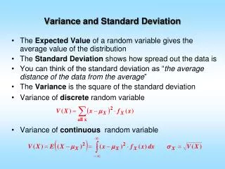
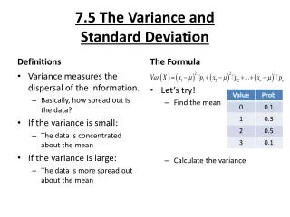
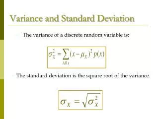
35. Variance of a Random Variable X • Suppose a random variable has the probability distribution and expected value E(X) = m • Then the variance of the random variable X is

36. Example • Find the variance of the random variable X whose probability distribution is Solution • The mean of the random variable X is given by Example 1, page 442

37. Example • Find the variance of the random variable X whose probability distribution is Solution • Therefore, the variance of X is given by Example 1, page 442

38. Standard Deviation of a Random Variable X • The standard deviation of a random variableX, s (pronounced “sigma”), is defined by where x1, x2, … , xn denote the values assumed by the random variableX and p1 =P(X = x1), p2 =P(X = x2), … , pn =P(X = xn).

39. Applied Example: Packaging • Let X and Y denote the random variables whose values are the weights of brand A and brand B potato chips, respectively. • Compute the means and standard deviations of X and Y and interpret your results. Applied Example 3, page 443

40. Applied Example: Packaging Solution • The means of X and Y are given by Applied Example 3, page 443

41. Applied Example: Packaging Solution • Therefore, the variance of X and Y are Applied Example 3, page 443

42. Applied Example: Packaging Solution • Finally, the standard deviations of X and Y are Applied Example 3, page 443

43. Applied Example: Packaging Solution • The means of X and Y are both equal to 16. • Therefore, the average weight of a package of potato chips of either brand is the same. • However, the standard deviation of Y is greater than that of X. • This tells us that the weights of the packages of brand B potato chips are more widely dispersed than those of brand A. Applied Example 3, page 443

44. Chebychev’s Inequality • Let X be a random variable with expected value m and standard deviations. • Then the probability that a randomly chosen outcome of the experiment lies between m – ks and m + ks is at least 1 – (1/k2) . • That is,

45. Applied Example: Industrial Accidents • Great Lumber Co. employs 400 workers in its mills. • It has been estimated that X, the random variable measuring the number of mill workers who have industrial accidents during a 1-year period, is distributed with a mean of 40 and a standard deviation of 6. • Use Chebychev’s Inequality to find a bound on the probability that the number of workers who will have an industrial accident over a 1-year period is between30 and 50, inclusive. Applied Example 5, page 445

46. Applied Example: Industrial Accidents Solution • Here, m = 40 and s= 6. • We wish to estimate P(30  X  50) . • To use Chebychev’s Inequality, we first determine the value of k from the equation m – ks = 30 or m + ks = 50 • Since m= 40 and s= 6, we see that k satisfies 40 – 6k = 30 and 40 + 6k = 50 from which we deduce that k = 5/3. Applied Example 5, page 445

47. Applied Example: Industrial Accidents Solution • Thus, the probability that the number of mill workers who will have an industrial accident during a 1-year period is between 30 and 50 is given by that is, at least 64%. Applied Example 5, page 445

48. 8.4 P(SFFF) = P(S)P(F)P(F)P(F) = p· q · q · q = pq3 P(FSFF) = P(F)P(S)P(F)P(F) = q· p · q · q = pq3 P(FFSF) = P(F)P(F)P(S)P(F) = q· q · p · q = pq3 P(FFFS) = P(F)P(F)P(F)P(S) = q· q · q · p = pq3 The Binomial Distribution

49. Binomial Experiment • A binomial experiment has the following properties: • The number of trials in the experiment is fixed. • There are two outcomes in each trial: “success” and “failure.” • The probability ofsuccess in each trial is the same. • The trials are independent of each other.

50. Example • A fair die is thrown four times. Compute the probability of obtaining exactly one6 in the four throws. Solution • There are four trials in this experiment. • Each trial consists of throwing the die once and observing the face that lands uppermost. • We may view each trial as an experiment with two outcomes: • A success (S) if the face that lands uppermost is a 6. • A failure (F) if it is any of the other five numbers. • Letting p and q denote the probabilities of success and failure, respectively, of a single trial of the experiment, we find that Example 1, page 453