Download
1 / 40
400 likes | 422 Views
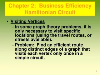
Chapter 2: Business Efficiency Hamiltonian Circuit. Visiting Vertices In some graph theory problems, it is only necessary to visit specific locations (using the travel routes, or streets available).

E N D
Chapter 2: Business EfficiencyHamiltonian Circuit Visiting Vertices In some graph theory problems, it is only necessary to visit specific locations (using the travel routes, or streets available). Problem: Find an efficient route along distinct edges of a graph that visits each vertex only once in a simple circuit. 1
Chapter 2: Business EfficiencyHamiltonian Circuit Applications: • Salesman visiting particular cities • Delivering mail to drop-off boxes • Route taken by a snowplow • Pharmaceutical representative visiting doctors 2
Hamiltonian Circuit Suppose we change the “Bridges of Konigsberg” problem so that we visit each land mass exactly once. Does this make the problem easier to do? R K O L YES!! 3
Chapter 2: Hamilton CircuitsOutline/Learning Objectives • To identify and model Hamilton circuit problems. • To use the following algorithms to determine the optimal route for a Traveling Salesman Problem. • Nearest Neighbor and Sorted Edges Algorithms • Minimum-Cost Spanning Trees • Kruskal’s Algorithm
(1805 – 1865) He was a renowned Irish mathematician and astronomer. He was a child prodigy. He could read English, Hebrew, Greek, and Latin by the time he was 4 yrs old. He became Professor of Astronomy at Trinity College in Dublin, Ireland when he was 23 yrs old. Sir William Rowan Hamilton 5
Hamiltonian Circuit: A path that starts and ends at the same vertex. Visits each vertex only once. Starting at vertex A, the tour can be written as ABDGIHFECA, or starting at E, it would be EFHIGDBACE. A different circuit visiting each vertex once and only once would be CDBIGFEHAC (starting at vertex C).
Circuits can start at any location. - Notice that we don’t care that we don’t use all the edges. Use wiggly edges to show the circuit. Unfortunately, there are no theorems that tell us whether or not a graph has a Hamilton Circuit. Hamiltonian Circuit: A different circuit visiting each vertex once and only once would be CDBIGFEHAC (starting at vertex C). Starting at vertex A, the tour can be written as ABDGIHFECA, or starting at E, it would be EFHIGDBACE. 7
Hamiltonian Circuit vs. Euler Circuits Euler circuit –A circuit that traverses each edge of a graph exactly once and starts and stops at the same vertex. Hamiltonian circuit– A path (shown by wiggly edges) that starts at a vertex of a graph and visits each vertex once and only once, returning to where it started. 8
Similarities Both forbid re-use. Hamiltonian didn’t reuse vertices. Euler didn’t reuse edges. Differences Hamiltonian is a circuit of vertices. Euler is a circuit of edges. Euler graphs are easy to spot (connectedness and even valence). Hamiltonian circuits are NOT as easy to determine upon inspection. Hamiltonian Circuit vs. Euler Circuits 9
Hamiltonian Circuit vs. Euler Circuits Find both an Euler and Hamilton Circuit Hamilton: one possible solution: AGFECDBA Euler: B and D have odd valences. Therefore, there is NO Euler Circuit. B A C D G E F 10
What are the possibleHamilton Circuits for this graph? One possible route: ABCDA or ADCBA Others: ABDCA or ACDBA ACBDA or ADBCA A D C B Notice that there are “mirror images” so then there are really only 3 different Hamilton circuits. 11
What are the possible Hamilton Circuits for this graph if we start at A? A ABCDA or ADCBA ABDCA or ACDBA ACBDA or ADBCA D C B When we start at A how many ways can we travel: If we choose B, how many ways can we travel: If we choose D, how many ways can we travel: 3 (B, D, C) 2 (D, C) 1 (C) This means that we can have 3 x 2 x 1 possible different combinations. This can be written as 3! How does 3 relate to the number of vertices? 3! = 6, but half were mirror images so 3!/2 = 3 would be the correct amount of unique Hamilton circuits. One less than 12
Unique Hamilton Circuits Principle of Counting for Hamiltonian Circuits For a complete graph of n vertices, there are (n - 1)! possible routes. Half of these routes are repeats, the result is: Possible unique Hamiltonian circuits are (n- 1)! / 2 Complete graph – A graph in which every pair of vertices is joined by an edge. • Fundamental Principle of Counting If there are a ways of choosing one thing, b ways of choosing a second after the first is chosen, c ways of choosing a third after the second is chosen…, and so on…, and z ways of choosing the last item after the earlier choices, then the total number of choice patterns is a×b × c × … × z. Example: Jack has 9 shirts and 4 pairs of pants. He can wear 9 × 4 = 36 shirt-pant outfits. 13
How many unique Hamilton circuits are there and name one. 5 vertices so there are 4! Hamilton circuits. 4! = 24 circuits 24/2 = 12 unique circuits (Be happy. I will only ask you to find one!) Example: ABCDEA C B D A E 14
Weighted Graphs • Vacation–Planning Problem • What would be the best route to take if you want to visit all 4 cities? • Hamiltonian circuit concept is used to find the best route (optimal route) that minimizes the total distance traveled to visit friends in different cities. (assume less mileage less gas minimizes costs) Hamiltonian circuit with weighted edges • Edges of the graph are given weights, or in this case mileage or distance between cities. • As you travel from vertex to vertex, add the numbers (mileage in this case). • Each Hamiltonian circuit will produce a particular sum. 15 Road mileage between four cities
Definitions • Weighted graph – has numbers assigned to an edge that can be thought of as cost, distance, or time. • Optimal solution – when a problem has various solutions and you pick the best solution for you. • Algorithm – A step-by-step description of how to solve a problem. Heuristic Algorithm – A “fast” method that doesn’t guarantee an optimal answer.
Weighted Graphs where the number of vertices in a complete graph are very large. Difficult to solve Hamiltonian circuits. This problem originated from a salesman determining his trip that minimizes costs (less mileage) as he visits the cities in a sales territory, starting and ending the trip in the same city. Many applications today: bus schedules mail drop-offs to post offices Candy machine coin pick-up routes UPS Running phone lines or cable Water lines Traveling Salesman Problem (TSP) 17
How can the TSP be solved? Computer program can find optimal route (not always practical). Exhaustive search called Brute Force Algorithm(Trees can be used) Heuristic methods can be used to find a “fast” answer, but does not guarantee that it is always the optimal answer. Nearest Neighbor Algorithm (NNA) Sorted Edges Algorithm (also known as “Cheapest Link”) Kruskal’s Algorithm (Minimum Spanning Trees) Traveling Salesman Problem (TSP) 18
Brute Force Algorithm – optimal algorithm that always works but inefficient. Creates a Hamilton Circuit. 2)Nearest-Neighbor Algorithm (NNA) – not optimal but efficient. Creates a Hamilton Circuit. 3)Sorted-Edges Algorithm - not optimal but efficient. Creates a Hamilton Circuit. 4) Kruskal’s Algorithmand Minimum Cost Spanning Trees - not optimal but efficient. Does NOT create a Hamilton Circuit. TSP Strategies for complete graphs 19
TSP Strategy Brute Force Algorithm • Algorithm(step-by-step process) for solving this airplane route problem CL • Generate all possible Hamiltonian tours (paths) using a table. • Add up the distances on the edges of each tour. • Choose the tour of minimum distance. S C M 20
TSP Strategy Brute Force Algorithm • Use the Brute Force Algorithm to determine the optimal Hamilton Circuit. 300 + 562 + 774 + 349 C,S,M,CL,C (or C,CL,M,S,C) 1,985 C,M,CL,S,C (or C,S,CL,M,C) 425 + 774 + 541 + 300 2,040 C,M,S,CL,C (or C,CL,S,M,C) 425 + 562 + 541 + 349 1,877 21
TSP Strategy Brute Force Algorithm The optimal Hamilton Circuit is: C,M,S,CL,C Chicago, Minn., St. Louis, Cleveland, and back to Chicago. 22
TSP Strategy Brute Force Algorithm and Trees Instead of creating a table, you create a tree. • This method begins by selecting a starting vertex, say Chicago, and making a tree-diagram showing the next possible locations. • In this example, the method of trees generated six different paths, all starting and ending with Chicago. However, only three are unique circuits. • At the end of each path put total weight. 23
TSP Strategy Brute Force Algorithm and Trees Definition: Tree – connected graph with NO circuits. 425 349 300 541 541 562 774 774 562 541 541 562 774 562 774 300 300 349 425 425 349 1877 2040 1985 2040 1985 1877
Use the Brute Force Algorithm to determine the optimal Hamilton Circuit. D 205 500 200 E 340 C 185 360 302 305 165 A B 320 How many Hamilton Circuits are there? How many are unique Hamilton Circuits? (5-1)! = 4! = 24 24/2 = 12 25
Use the Brute Force Algorithm to determine the optimal Hamilton Circuit. 320+305+500+205+302 1332 1632 ABCDEA ADBCEA 320+305+500+205+302 1355 1250 ABCEDA ADBECA 320+305+500+205+302 1662 1510 ABDCEA ADCEBA 1425 1457 ABDECA ADCBEA 1550 1220 ABEDCA ADEBCA 1355 1510 ADECBA ABECDA 1457 1372 ACBDEA AEBCDA 1220 1527 ACBEDA AEBDCA 1527 1332 ACDBEA AECBDA 1550 1662 ACDEBA AECDBA 1425 1372 ACEDBA AEDBCA 26 1250 1632 ACEBDA AEDCBA
Use the Tree method to determine the optimal Hamilton Circuit. A E D C B D C B E C B E D B E D C C B B D C B B D B B D D C C D C E E C E E E E D B C B D D C B C B E C E B E C D E E B D E D C D A A A A A A A A A A A A A A A A A A A A A A A A
TSP Strategy Nearest Neighbor Algorithm (NNA) Pick a “home” city (or vertex). Travel from vertex to vertex by always choosing the next vertex that can be reached quickest (least miles), that has not already been visited. When all vertices have been visited, the tour returns home. NNA starting at vertex B Hamiltonian Circuit: B-C-A-D-E-B NNA starting at vertex A Hamiltonian Circuit: A-B-C-E-D-A 28
Use the NNA to determine the optimal Hamilton Circuit. D 205 500 200 E 340 C 185 360 302 305 165 A B 320 D B E C 1250 185 200 165 340 360 29
TSP StrategySorted Edges Algorithm Start by sorting, or arranging, the edges in order of increasing weight (smallest to largest mileage between cities). Choose an edge with lowest weight That will NOT result in three edges meeting at a vertex That will NOT close up a path that doesn’t include all vertices Repeat #2 until all vertices are used. From last vertex, return to start D 205 500 200 E 340 C 185 360 302 305 165 A B 320 30
TSP StrategySorted Edges Algorithm • Arrange edges in order low to high: BE 165 AD 185 BD 200 ED 205 AE 302 BC 305 AB 320 EC 340 AC 360 DC 500 D 205 500 200 E 340 C 185 360 302 305 165 A B 320 31
Step 2) Choose an edge with lowest weightThat will NOT result in three edges meeting at a vertexThat will NOT close up a path that doesn’t include all verticesStep 3) Repeat #2 until all vertices are used.Step 4) From last vertex, return to start BE 165 AD 185 BD 200 ED 205 AE 302 BC 305 AB 320 EC 340 AC 360 DC 500 D E C circuit circuit 3 edges A 3 edges B Not needed Total: 1250 Hamilton circuit: ADBECA or ACEBDA
Recall the Tree method to determine the optimal Hamilton Circuit. A E D C B D C B E C B E D B E D C C B B D C B B D B B D D C C D C E E C E E E E D B C B D D C B C B E C E B E C D E E B D E D C D A A A A A A A A A A A A A A A A A A A A A A A A
Definition: Spanning Tree – is a subgraph that connects all vertices and has NO circuits. Therefore, you don’t go back to A at the end. Each branch of a tree is a “spanning tree”
TSP Strategy -Spanning Trees Spanning trees look more like this: D A E B C C Spanning trees don’t really look like this though. E A B D 35
TSP Strategy -Spanning Trees D D Original: Example 1) E C E C A B Example 2) D A E C B A B 36
Minimum-Cost Spanning Trees and Kruskal's Algorithm • Goal of minimum-cost spanning tree: Create a tree that links all the vertices together and achieves the lowest cost to create. • The cost of the tree is the sum of the weights on the edges. 37
Minimum-Cost Spanning Trees and Kruskal's Algorithm Kruskal’s Algorithm — Developed by Joseph Kruskal (AT&T research). Add links in order of cheapest cost according to the rules: No circuit is created (no loops). If a circuit (or loop) is created by adding the next largest link, eliminate this largest (most expensive link)—it is not needed. Every vertex must be included in the final tree. 38
TSP StrategyMinimum-Cost Spanning Trees D Kruskal's Algorithm 1) On every step mark the cheapest unmarked edge. - See that the marked edges do not form circuits (loops). 2) Repeat while possible until all vertices are connected. 205 500 200 E 340 C 185 360 302 305 165 A B 320 Total distance: 855 miles 39
Minimum-Cost Spanning Trees and Kruskal's Algorithm • The diagram shows the cost to build the connection from each vertex to all other vertices (connected graph). • Costs (in millions of dollars) of installing Pictaphone service among five cities • The cost of redirecting the signal may be small compared to adding another link. Example: What is the cost to construct a Pictaphone service (telephone service with video image of the callers) among five cities? Total cost: $2.55 million 40