Download
1 / 52
520 likes | 665 Views
Application: Process Relations. Some algorithms require that sub processes (tasks) are executed in a certain order, because they use data from each other Example: get dressed In which order should I don my clothes? Such an order is known as a topological sort. Tee-shirt before shirt

E N D
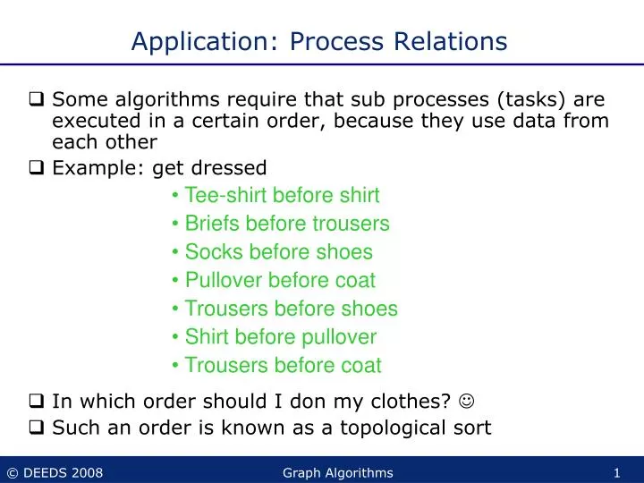
Application: Process Relations • Some algorithms require that sub processes (tasks) are executed in a certain order, because they use data from each other • Example: get dressed • In which order should I don my clothes? • Such an order is known as a topological sort • Tee-shirt before shirt • Briefs before trousers • Socks before shoes • Pullover before coat • Trousers before shoes • Shirt before pullover • Trousers before coat
Tee-shirt Shirt Pullover Coat Shoes Briefs Trousers Socks Application: Process Dependencies • Tee-shirt before shirt • Briefs before trousers • Socks before shoes • Pullover before coat • Trousers before shoes • Shirt before pullover • Trousers before coat Are these the only rules?
Tee-shirt Shirt Pullover Coat Shoes Briefs Trousers Socks Application: Process Relations Transitivity Relation??
Partial Order A partial order is a relation that (informally) expresses: For any two objects holds that either... • The object relate with a “greater/smaller than”, “before/after” type relation • ...or the two objects are incomparable (shirt or socks first?) • So what is so partial about the ordering?
p. 1075 Acyclic Graphs and Partial Order • Definition: A partial Order (M, ) consists of a set M and a irreflexive, transitive, antisymmetric order relation () • Cormen’s definition is reflexive, transitive, antisymmetric • In a partial order, some elements can be incomparable • Acyclic graphs specify partial orders : Let • G = (V,E) be an acyclic, directed graph • G+ = (V,E+) be the corresponding transitive closure • The partial order ( V, G ) is defined as: vi G vj ( vi, vj ) E+
Transitive Closure • There are unfortunately multiple definitions for the transitive closure… • There is another definition, where G* is called the transitive closure(Cormen for instance) • G* = (V,E*), where E* = E+ { (v,v) | v V } • G* sometimes also known as the reflexive transitive closure • We will use: G+ = transitive closure (Wegegraph in German) • For all definitions: use the one on the slides! Also for the exam!
Maths… Let be a relation (on for example ) • Reflexive (=,≤,≥) • Irreflexive (<) • Antisymmetric (≤,≥) • Transitive (=,<, ≤,≥)
Example E+ = { (v1, v3), (v1, v4), (v1, v5), (v1, v6), (v1, v7), (v2, v3), (v2, v4), (v2, v5), (v2, v6), (v2, v7), (v3, v4), (v3, v5), (v3, v6), (v3, v7), (v4, v6), (v5, v6), (v5, v7) } Graph G
Deadlock • Test: find cycles = test for partial order • How do we do this? Example (fictive :-) Assume: “The coat should be put on before the shirt” Tee-shirt Shirt Pullover Coat Shoes Briefs Trousers Socks
Tee-shirt Shirt Pullover Coat p. 549 Shoes Briefs Trousers Socks Topological Sort • Topological sort order: a sequence of objects that adhere to a partial order Example: Tee-shirt Shirt Pullover Briefs Trousers Socks Shoes CoatorBriefs Tee-shirt Trousers Shirt Socks Shoes Pullover Coat
Topological Sort • Definition: The arrangement of elements mi of a partially ordered set (M,) in a sequence m1, m2, ..., mk is called topological sort if for any two indices i and j with 1 i < j k the following holds: • Either mi mj or • mi and mj are incomparable • Topological Sort is a “linearization” of elements, that is compatible with partial order • Visualized as a graph: Arrangement of vertices on a horizontal line so that all edges go from left to right v7 v1 v4 v3 v1 v2 v5 v4 v7 v3 v6 v6 v2 v5
Finding of a Topological Sort • Finding a topological sort can be done using graph algorithms • Starting point: • Determine the acyclic graph G that corresponds to (M,). • Two possible approaches: • (top down): As long as G is not empty... • Find a vertex v with incoming degree 0 • Delete v from G together with its corresponding edges • Save the deleted vertices in this order • (bottom up): • Starting from the vertex with incoming degree 0, start a DFS traversal. • Assign reverse “visit numbers” beginning with the “deepest” vertex.
1 2 3 4 5 6 7 Example: top down • Find a vertex with d-(v) = 0 • Delete from G vertex v and all incident edges • Save the deleted vertices in this order • Repeat steps 1 to 3 until G is empty Graph G Possible topological sorts: 1, 2, 3, 4, 5, 6, 7 2, 1, 3, 5, 4, 6, 7 1, 2, 3, 4, 5, 7, 6 2, 1, 3, 5, 7, 4, 6 ...
Cost: top down • In worst case you always find the next vertex with in-degree 0 last O(|V|2) Example: v4 v3 v2 v1
Example: bottom up (DFS) Given: acyclic Graph G = ( V, E ) Find: topological sort TS[v] for all v V for ( all v V ) { v.unvisit( ); } /* initialization */ z = |V|; /* maximum number in TS */ for ( all v V ) { if ( d-(v) == 0 ) v.topSort( ); /* all starting vertices */ } void topSort( ) { /* DFS Traversal */ this.visit( ); for ( all k‘ this.neighbors( ) ) if ( k‘.unvisited( ) ) k‘.topsort(); TS[ v ] = z; /* Assignment of TS at the end*/ z--; }
1 2 3 4 5 6 7 Example 2 1 • Vertices are named “backwards” while ascending from DFS recursion. • Sorting order: 2 1 3 5 7 4 6 3 6 4 7 5
Cost: bottom up • Consists of • Search for nodes with in-degree 0 O (|V|) • DFS on the corresponding subgraphs O (|V|+|E|) • Total cost O(max (|V|,|E|) • A bit more complicated, but “better” than top down
Side kick: Total Order • There is not only partial order • Total order is a partial order where all elements in the set M are pair wise comparable • For example: ‘≤’ and ‘≥’ • But not: “is a child of” over all Germans • Where could these orders be useful? • Deadlock detection in concurrent programs • Message ordering and consistency in distributed computing
Application: Cable Routing • The possible cable channels are defined by the channels • Goal: every computer should be reachable
Solution: Spanning Tree • Model the problem as a graph • Create a spanning tree • As long there is a cycle left: • Remove an edge from a cycle 3 1 2 4 5 6 7 8
Ch. 23 Spanning Trees • Definition: A subgraph B is a spanning tree of a graph G, if there are no cycles in B and B contains all vertices in G • It is not difficult to build a spanning tree of a connected graph: • If G is acyclic, then G is a spanning tree itself. • If G contains cycles, delete an edge from the cycle (the graph stays connected) and repeat the procedure until there are no more cycles.
Spanning Trees (2) • Edges in G and B are called branches • Edges in G and not in B are called chords • A graph with n vertices and e edges has n-1 branches and e - n + 1 chords • The spanning tree of a graph is not unique • All spanning trees of a graph can be systematically constructed by means of an acyclic exchange: • Find any spanning tree B of G • Add a chord to B (that leads to a cycle in B) • Delete another edge from B
Example • B1, B2, B3 - all spanning trees of G Graph G Chords (edges in G and not in B) Branches (edges in B) B1 B3 B2
Application: Cable Routing • The green numbers indicate the lengths of the cables • How do we find the cheapest (shortest) routing?
Minimum Spanning Trees • We look at spanning trees of labeled graphs where edges are labeled with c. • Definition: The weight c of a spanning tree B = (V,E) is the sum of the weights of its branches, i.e. c(B) = eE c(e) . • Definition: A spanning tree B = ( V, E ) is called the minimum spanning tree of graph G, if for any B‘ = ( V, E‘ ) of G the following holds: c(B) c(B‘)
Example 7 • c(B1) = 12, c(B2) = 15, c(B3) = 16 • B1 is minimum spanning tree of G labeled graph G Chord 3 4 Branch 5 B1 B2 B3
Finding Minimum Spanning Trees • Idea: greedy-principle, i.e. decide on the basis of the knowledge currently available and never revise the decision. • Efficient in contrast to methods that sample solutions, evaluate and revise them if necessary. Given: Graph G = ( V, E ) labeled with c Find: minimum spanning tree T‘ = (V, E‘) of G. E‘ = { }; while (not yet finished) { choose an appropriate edge e E; E‘ = E‘ { e } }
Kruskal‘s Algorithm • Sampling of edges according to the principle of the lowest weight. • Sort edges according to their weights. • Choose the edge with the lowest weight. • If E‘ { e } results in a cycle, drop e. e‘ Observation: If there is a cycle, it is pointless to leave e in the tree and to drop another edge e‘, because c(e‘) < c(e). e
Example: Kruskal Sorting: (1, 2) (3, 4) (2, 3) (3, 6) (4, 6) (1, 5) (5, 6) (5, 7) (4, 8) (7, 8) (2, 7) (1, 7) 5 6 3 1 2 5 7 22 9 19 4 5 8 14 11 14 16 6 7 8 Needed length: 60m
Kruskal‘s Algorithm: Complexity • The complexity comes from • Cost for sorting the edges (possible with O(|E| log |E|)) • Cost for testing for cycles(also O(|E| log |E|)) • Total: O(|E| log |E|)
Prim‘s Algorithm • Enhancement of Kruskal‘s Algorithm by Prim (sometimes Dijkstra is declared as the author): Given: G = ( V, E ) labeled with c Find: minimum spanning tree T = ( V, E‘ ) of G V‘ = { arbitrary start vertex v V } for (int i = 1; i |V| - 1; i++ ) { e = edge (u,v) E with u V‘ and v V‘ and minimum weight c V‘ = V‘ { v }; E‘ = E‘ { e } }
Example 5 6 3 1 2 5 7 22 9 19 4 5 8 14 11 14 16 6 7 8
Analysis • (Efficient) cycle testing is an integral part of Kruskal‘s algorithm: • Interconnecting two different connected components of a graph by an edge does not lead to a cycle • The vertices belonging to the new edge must be located in different components • Upon the assembly, the smaller component is added to the larger one • Works with appropriate data structures inO( |E| log |V| ) time
Ch. 24 Path Finding Problems • Finding certain paths in a graph • Distinct boundary conditions lead to different problems: • (un)directed graph • Type of weights (only positive or also negative weights, bounded weights?) • Shortest vs. longest path • Path existence (Number of Paths) • Start and end vertex: • Paths between a specified pair of vertices • Paths between a start vertex and all others • Paths between every pair of vertices
1. Approach: Brute force • Brute force: • The simplest way • Try all possible paths • Cost: normally exponential • Worst case: Complete graph • n cities (n-1)! Different paths with (n-1) edges each complexity O(nn!)
1. Approach: Brute force • 5 Nodes: 96 paths • 10 Nodes : 3.265.920 paths • 100 Nodes : 92392953289504711154882246467704033485808808581737805253907034256265423993297616452852049336394953103391160941618951520668673358807695360000000000000000000000 paths • All 12903 communities in Germany:
2. Approach: Ants How do ants find a short path from I to O? Solution: search concurrently! • Instead of testing, find all ways at once
Shortest Path • Definition: The weightof a path p = v1, v2, ..., vk in a graph G = ( V, E ) with edges labeled with c, is the sum of the weights of its constituent edges, e.g.: c(p) = c(( vi, vi+1 )) • Definition: The shortest path between two vertices u and v in G is the path with minimum weight • The weight of the shortest path is called the distance between u and v • In non-weighted graphs, c(p) = |p| k-1 i=1
Example 7 d c • All paths from a to d: p1 = a, b, c, d p2 = a, b, d • Shortest path from a to d: p2 (weight 9) • Shortest path from e to f: p3 = e, f (weight 2) • Shortest path from a to e? e 3 4 2 a b f 5
Single Source Problem • single source shortest path: Given a graph G = ( V, E ), we want to find a shortest path from a source vertex s V to all other vertices v V. • BFS-based algorithm (by Moore): uses length attribute D of a vertex to keep the distance (as number of hops). for ( all v V ) { v.D = } /* Initialization */ Queue Q = new Queue( ); Q.enqueue( s ); s.D = 0; i = 0; /* s is source vertex */ while ( !Q.empty( ) ) { w = Q.dequeue( ); if ( w.D == i ) i++; /* next level in BFS */ for ( all v w.neighbours( ) ) { if ( v.D == ) { v.D = i; Q.enqueue(v); } } }
Example “Wave propagation” in the graph
Analysis • Moore‘s Algorithm has the same time complexity as BFS, i.e. O( max( |E|, |V| )). • The algorithm does not work for weighted edges • Enhancement by Dijkstra was published 1959!
Dijkstra‘s Algorithm • single source shortest path with arbitrary positive edge weights, start vertex s • Correctness is based on the principle of optimality: For any shortest path p = v1, ..., vk from v1 to vk, each subpath p‘ = vi, ..., vj with 1 i < j k is a shortest path between vi and vj. • Proof: • Assume that this does not hold, i.e. there is a shorter path p‘‘ p‘ between vi and vj. • Then, there exists a shorter path between v1 and vk by exchanging subpath p‘ with p“.
Dijkstra‘s Algorithm (2) • Each vertex belongs to one of the categories M1, M2, M3. • Extract vertex v from M2 to which there is a minimal edge between M1 und M2 and insert v in M1 (principle of optimality). • For each vertex that was moved to M1, move its successors to M2. M3 M2 M1 s u v selected vertices not reached vertices marginal vertices
Dijkstra‘s Algorithm (3) • More precisely: Divide the vertices in the graph into three subsets: • M1 contains all vertices v, for which shortest paths between s and v are already known. • M2 contains all vertices v, that are reachable via an edge from a vertex in M1. • M3 contains all other vertices. • Invariant: denote sp(x,y) as the shortest path from x to y. Then, the following holds: • For all shortest paths sp(s,u) and all edges (u,v) c(sp(s,u)) + c((u,v)) c(sp(s,v)) • For at least one shortest path sp(s,u) and one edge (u,v) c(sp(s,u)) + c((u,v)) = c(sp(s,v))