Download
1 / 31
310 likes | 438 Views
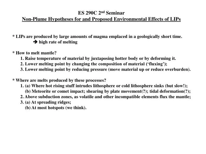
ES 290C 2 nd Seminar Non-Plume Hypotheses for and Proposed Environmental Effects of LIPs. * LIPs are produced by large amounts of magma emplaced in a geologically short time. high rate of melting * How to melt mantle?

E N D
ES 290C 2nd Seminar Non-Plume Hypotheses for and Proposed Environmental Effects of LIPs * LIPs are produced by large amounts of magma emplaced in a geologically short time. high rate of melting * How to melt mantle? 1. Raise temperature of material by juxtaposing hotter body or by deforming it. 2. Lower melting point by changing the composition of material (‘fluxing’); 3. Lower melting point by reducing pressure (move material up or reduce overburden). * Where are melts produced by these processes? 1. (a) Where hot rising stuff intrudes lithosphere or cold lithosphere sinks (but slow!); (b) Meteorite or comet impact; shearing by plate movement(?); tidal deformation(?); 2. Above subduction zones, as volatile and other incompatible elements flux the mantle; 3. (a) At spreading ridges; (b) At most hotspots (we think).
Various Proposed Hotspot Volcanism Mechanisms * Subduction melting in back-arc extending environment under continent (OPB!). * Impact melting ( subsequent decompression melting). * Shear melting ( subsequent decompression melting). * Decompression melting: 1. Plumes that (a) inherit excess temperature from thermal boundary layer where they started; (b) crack or weaken lithosphere, then rises and decompresses more; (c) originate in more fertile material (undepleted mantle, eclogite, ...). 2. Cracks that propagate to produce volcanic chains and tracks (a) with lithosphere moving over local melting anomaly; (b) without local melting anomaly (self-propagating over hot lithosphere). 3. Pull-apart zones over unusually hot or fertile asthenosphere (to exceed MORB rate). 4. Lithospheric steps that promote edge convection. 5. Local upwelling and diapirs produced by delamination.
SHEAR MELTING Shaw, H.R., and Jackson, D.E., 1974, Linear island chains in the Pacific: Result of thermal plumes or gravitational anchors?: Journal of GeophysicalResearch, v. 78, p. 8634–8652.
Impact Melting (A) Theoretical correlation of impact melt volume versus crater diameter for terrestrial impact craters (sloping line) with locus of terrestrial impact melt below this line (after Grieve and Cintala 1992). Also shown is the melt volume typical of a LIP (horizontal dashed line at 106 km3). (B) Hypothetical increase in impact melt volume above the theoretical sloping line, due to additional decompression melting of lithospheric mantle for large crater diameters, not precisely determined (see Jones et al. 2002, 2003). From Jones, Elements, 2005.
(A) Shocked quartz from Tertiary breccia, Antrim, Northern Ireland. Field of view 2.5 mm, plane polarized light (PPL). (B)–(D) From Tertiary spherule bed, Nuussuaq, West Greenland (after Jones et al. 2005b). (B) Impact melt glass spherules, field of view 2.5 mm (PPL). (C) Skeletal quench-textured Ni-spinel occurring as radiating “christmas trees” (PPL). (D) Detail of (C). Backscattered electron image (width ~50 µm) showing Ni-spinel crystals, which have an irregular core of nearly pure Ni metal.
Discrete alternating hotspot islands formed by interaction of magma transport and lithospheric flexure Hieronymus & Bercovici, 1999, Nature 397, 604-607 Figure 2 Theoretical model of discrete islands formed on a lithospheric plate moving over a mantle hotspot. In the lithospheric reference frame, the hotspot starts at x =70 km, y =110 km and moves to the right at velocity v =10cm/yr, causing a line of single volcanoes. When the hotspot reaches x =470 km, the relative direction of plate motion changes by 45 deg, causing a transition to a dual line of volcanoes (see text for discussion). Figure 1 Sketch of the influence of flexural stresses on fracture formation. Fractures form where the magma pressure due to the plume is greater than the sum of compressive stresses due to flexure and the tensile strength of the lithosphere. Once magma pathway is established, the fracture is kept open in an environment of increasing flexural stresses by erosion of the fracture walls.
Non-hotspot formation of volcanic chains: control of tectonic and flexural stresses on magma transport C.F. Hieronymus, D. Bercovici, 2000,Earth and Planetary Science Letters 181, 539-554
Young, thin elastic lithosphere
Older, thicker elastic lithosphere (thin-plate elastic theory no longer applicable)
Pull-apart Volcanism Unless asthenosphere is unusually hot or unusually fertile it is difficult to get flood- basalt eruption rates.
King & Anderson, 1998 King & Anderson, 1995 EDGE CONVECTION CONTINENT OCEAN HOT HOT CONTINENT OCEAN
1 cm/yr 0.0 instabilities 0.1 1 cm/yr 0.01 0.001 Fig. 2. Average velocity time series from the three calculations in Fig. 1: pert D 0.1 (solid), pert D 0.01 (dashed), pert D 0.001 (short dash), pert D 0.0 (dotted). Fig. 3. Flow field for edge-driven models with Imposed Couette side-wall boundary conditions. (A) 10 mm=yr to the left; (B) 10 mm=yr to the right. All other parameters are identical to the calculations in Fig. 1C.
DELAMINATION Where in the world did the ocean crust go?(Anderson, 1989, Physics Today) Figure 3. The neutral density profile of the crust and mantle. The materials of the crust and mantle are arranged mostly in order of increasing density. A” is the region of over-thickened crust that can transform to eclogite and become denser than the underlying mantle. C’ is the top part of the transition region. Eclogites having STP densities between 3.6 and 3.7 g/cc may be trapped in C’. Eclogites and peridotites have similar densities in this interval but different seismic velocities. In C”, MORB-eclogite and low-MgO arc-eclogites reach density equilibration. Trapped eclogite and dense eclogite sinkers can be low velocity zones. The order approximates the situation in an ideally chemically stratified mantle, except for the region just below the continental Moho where potentially unstable lower crustal cumulate material is formed. In such a stably stratified structure the temperature gradient will be greater than the adiabatic gradient. TZ = transition zone; Lhz = lherzolite; Coe = coesite; St = stishovite. Anderson, Elements, 2005
Anderson, Elements, 2005 Figure 2. Melting relations in dry lherzolite and eclogite based on laboratory experiments. The dashed line is a reference 1300°C mantle adiabat. Eclogite will melt as it sinks into normal-temperature mantle, and upwellings from the shallow mantle will extensively melt any entrained gabbro and eclogite. Eclogite will be about 70% molten before dry lherzolite starts to melt (compiled by J. Natland, personal communication). The two vertical lines separate the gabbro field from the eclogite field (in between is the mixed phase region).
? Saunders, Elements, 2005 ?
Fig. 1. Extinction rate versus time (multiple-interval marine genera: modified from Sepkoski, (1996) to reflect radiometric age constraints on stratigraphic boundaries) compared with eruption ages of continental flood basalt provinces. Three of the most severe extinctions, the P–Tr, the Tr–J and the K–T, correspond with eruption of the Siberian Traps, Central Atlantic Magmatic Province and Deccan Traps, respectively. Evidence of impact (*) has also been reported at these times (Alvarez et al., 1980; Becker et al., 2001; Olsen et al., 2002a; Basu et al., 2003). The K–Tcrater is ~180 km in diameter; for the P–Tr and Tr–J boundaries, the size (and indeed existence) of any impact is not confirmed. The end-Guadalupian extinction (~259 Ma) coincides with eruption of the Emeishan Traps (Zhou et al., 2002), but no evidence for impact has been noted for this boundary. Oceanic plateaus may also have had profound environmental consequences (e.g., Kerr, 1998). Selected oceanic plateaus are therefore included on this figure, but as text only, because the preservational bias of the geological record towards younger examples would otherwise render the diagram misleading. SP: Sorachi Plateau, Japan; KP: Kerguelen Plateau; OJP: Ontong Java Plateau; CP: Caribbean-Colombian Plateau. (White and Saunders, Lithos 79, 299-316)
Flow chart showing suggested chain of environmental events caused by the eruption of large igneous provinces. The chart is colour coded to distinguish between observed facts (yellow), inferred consequences for which there is overwhelming geological evidence (purple) and other, somewhat more tentatively inferred consequences for which there is not always supporting evidence (red).