Space-for-time tradeoffs

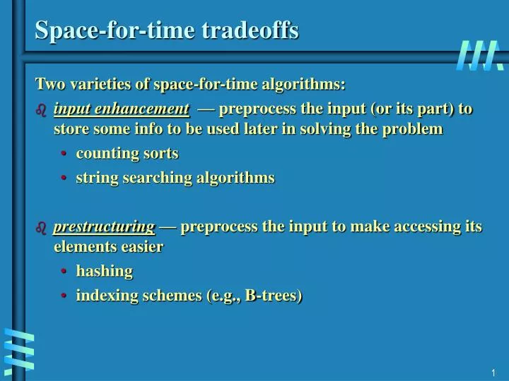
1. Space-for-time tradeoffs Two varieties of space-for-time algorithms: • input enhancement— preprocess the input (or its part) to store some info to be used later in solving the problem • counting sorts • string searching algorithms • prestructuring— preprocess the input to make accessing its elements easier • hashing • indexing schemes (e.g., B-trees)

2. Review: String searching by brute force pattern: a string of m characters to search for text: a (long) string of n characters to search in Brute force algorithm Step 1 Align pattern at beginning of text Step 2 Moving from left to right, compare each character ofpattern to the corresponding character in text until either all characters are found to match (successful search) or a mismatch is detected Step 3 While a mismatch is detected and the text is not yet exhausted, realign pattern one position to the right and repeat Step 2

3. String searching by preprocessing Several string searching algorithms are based on the input enhancement idea of preprocessing the pattern • Knuth-Morris-Pratt (KMP) algorithm preprocesses pattern left to right to get useful information for later searching • Boyer -Moore algorithm preprocesses pattern right to left and store information into two tables • Horspool’s algorithm simplifies the Boyer-Moore algorithm by using just one table

4. Horspool’s Algorithm A simplified version of Boyer-Moore algorithm: • preprocesses pattern to generate a shift table that determines how much to shift the pattern when a mismatch occurs • always makes a shift based on the text’s character c aligned with the last character in the pattern according to the shift table’s entry for c

5. How far to shift? Look at first (rightmost) character in text that was compared: • The character is not in the pattern .....c...................... (c not in pattern) BAOBAB • The character is in the pattern (but not the rightmost) .....O...................... (O occurs once in pattern) BAOBAB .....A...................... (A occurs twice in pattern) BAOBAB • The rightmost characters do match .....B...................... BAOBAB

6. A B C D E F G H I J K L M N O P Q R S T U V W X Y Z 1 2 6 6 6 6 6 6 6 6 6 6 6 6 3 6 6 6 6 6 6 6 6 6 6 6 Shift table • Shift sizes can be precomputed by the formula distance from c’s rightmost occurrence in pattern among its first m-1 characters to its right end t(c) = pattern’s length m, otherwise by scanning pattern before search begins and stored in atable called shift table • Shift table is indexed by text and pattern alphabet Eg, for BAOBAB:

7. _ 6 A B C D E F G H I J K L M N O P Q R S T U V W X Y Z 1 2 6 6 6 6 6 6 6 6 6 6 6 6 3 6 6 6 6 6 6 6 6 6 6 6 Example of Horspool’s alg. application BARD LOVED BANANAS BAOBAB BAOBAB BAOBAB BAOBAB (unsuccessful search)

8. Boyer-Moore algorithm Based on same two ideas: • comparing pattern characters to text from right to left • precomputing shift sizes in two tables • bad-symbol table indicates how much to shift based on text’s character causing a mismatch • good-suffix table indicates how much to shift based on matched part (suffix) of the pattern

9. Bad-symbol shift in Boyer-Moore algorithm • If the rightmost character of the pattern doesn’t match, BM algorithm acts as Horspool’s • If the rightmost character of the pattern does match, BM compares preceding characters right to left until either all pattern’s characters match or a mismatch on text’s character c is encountered after k > 0 matches text pattern bad-symbol shift d1=max{t1(c ) - k, 1} c k matches

10. Good-suffix shift in Boyer-Moore algorithm • Good-suffix shift d2 is applied after 0 < k < m last characters were matched • d2(k) = the distance between matched suffix of size k and its rightmost occurrence in the pattern that is not preceded by the same character as the suffixExample: CABABA d2(1) = 4 • If there is no such occurrence, match the longest part of the k-character suffix with corresponding prefix; if there are no such suffix-prefix matches, d2 (k) = mExample: WOWWOW d2(2) = 5, d2(3) = 3, d2(4) = 3, d2(5) = 3

11. Good-suffix shift in the Boyer-Moore alg. (cont.) After matching successfully 0 < k < m characters, the algorithm shifts the pattern right by d = max {d1, d2} where d1=max{t1(c) - k, 1} is bad-symbol shift d2(k) is good-suffix shift

12. Boyer-Moore Algorithm (cont.) Step 1 Fill in the bad-symbol shift table Step 2 Fill in the good-suffix shift table Step 3 Align the pattern against the beginning of the text Step 4 Repeat until a matching substring is found or text ends: Compare the corresponding characters right to left. If no characters match, retrieve entry t1(c) from the bad-symbol table for the text’s character c causing the mismatch and shift the pattern to the right by t1(c).If 0 < k < m characters are matched, retrieve entry t1(c) from the bad-symbol table for the text’s character c causing the mismatch and entry d2(k) from the good-suffix table and shift the pattern to the right by d = max {d1, d2}where d1=max{t1(c) - k, 1}.

13. _ 6 A B C D E F G H I J K L M N O P Q R S T U V W X Y Z 1 2 6 6 6 6 6 6 6 6 6 6 6 6 3 6 6 6 6 6 6 6 6 6 6 6 Example of Boyer-Moore alg. application B E S S _ K N E W _ A B O U T _ B A O B A B S B A O B A B d1 = t1(K) = 6 B A O B A B d1 = t1(_)-2 = 4 d2(2) = 5 B A O B A B d1 = t1(_)-1 = 5 d2(1) = 2 B A O B A B (success)

14. Boyer-Moore example from their paper Find pattern AT_THAT in WHICH_FINALLY_HALTS. _ _ AT_THAT

15. Hashing • A very efficient method for implementing a dictionary, i.e., a set with the operations: • find • insert • delete • Based on representation-change and space-for-time tradeoff ideas • Important applications: • symbol tables • databases (extendible hashing)

16. Hash tables and hash functions The idea of hashing is to map keys of a given file of size n into a table of size m, called the hash table,by using a predefined function, called the hash function, h: K  location (cell) in the hash table Example: student records, key = SSN. Hash function: h(K) = K mod m where m is some integer (typically, prime) If m = 1000, where is record with SSN= 314159265 stored? Generally, a hash function should: • be easy to compute • distribute keys about evenly throughout the hash table

17. Collisions If h(K1) = h(K2), there is a collision • Good hash functions result in fewer collisions but some collisions should be expected (birthday paradox) • Two principal hashing schemes handle collisions differently: • Open hashing– each cell is a header of linked list of all keys hashed to it • Closed hashing • one key per cell • in case of collision, finds another cell by • linear probing: use next free bucket • double hashing: use second hash function to compute increment

18. Open hashing (Separate chaining) Keys are stored in linked lists outside a hash table whose elements serve as the lists’ headers. Example: A, FOOL, AND, HIS, MONEY, ARE, SOON, PARTED h(K) = sum of K ‘s letters’ positions in the alphabet MOD 13 0 1 2 3 4 5 6 7 8 9 10 11 12 A AND MONEY FOOL HIS ARE PARTED SOON Search for KID

19. Open hashing (cont.) • If hash function distributes keys uniformly, average length of linked list will be α = n/m. This ratio is called load factor. • Average number of probes in successful, S, and unsuccessful searches, U: S 1+α/2, U = α • Load α is typically kept small (ideally, about 1) • Open hashing still works if n > m

20. Closed hashing (Open addressing) Keys are stored inside a hash table. 0 1 2 3 4 5 6 7 8 9 10 11 12

21. Closed hashing (cont.) • Does not work if n > m • Avoids pointers • Deletions are not straightforward • Number of probes to find/insert/delete a key depends on load factor α = n/m (hash table density) and collision resolution strategy. For linear probing: S = (½) (1+ 1/(1- α)) and U = (½) (1+ 1/(1- α)²) • As the table gets filled (α approaches 1), number of probes in linear probing increases dramatically: