A Genetic Algorithm for the Weapon to Target Assignment Problem
A Genetic Algorithm for the Weapon to Target Assignment Problem. Matthias Chan 7 August 2009. Introduction. Weapon to Target Assignment (WTA) problem is to minimize the expected lethality of a system by optimally assigning weapons to targets which threaten assets of interest

A Genetic Algorithm for the Weapon to Target Assignment Problem
E N D
Presentation Transcript
A Genetic Algorithm for the Weapon to Target Assignment Problem Matthias Chan 7 August 2009
Introduction • Weapon to Target Assignment (WTA) problem is to minimize the expected lethality of a system by optimally assigning weapons to targets which threaten assets of interest • In its most general form, WTA is an NP-complete problem • There are no exact algorithms which are “efficient,” therefore must rely on heuristic algorithms • Performance analysis of heuristic algorithm, in terms of accuracy and computational efficiency, is shown when compared to a greedy algorithm and brute-force solution • Heuristic algorithm studied was the Genetic Algorithm (GA)
WTA – Pictorial (1 of 2) Success! Weapons Targets Assets
WTA – Pictorial (2 of 2) This is a static WTA problem All assignments are done at one time, in pictorial, weapons are assigned one at a time for clarity in assignment matrix 3 Weapons (W) 1 3 2 Targets (T) 1 4 If we number the weapons and targets accordingly, the following assignments are shown in the assignment matrix, x 2 Target 1 2 3 Weapon 4 3 2 1 0 0 1 0 0 0 0 1 Note that: x = 0 0 0 1 0 1 0 0
General WTA Problem Formulation Given • T targets and W weapons • Lethality probability of target j • Pl(j) for j = 1,…,T • Probability of kill of assigning weapon i to target j • Pk(i, j) for i = 1,…,W and j = 1,…,T • Assignment of weapon i to target j is represented by a binary variable x find the weapon to target assignment that minimizes the cost function subject to the constraint that a weapon can only be fired at one target
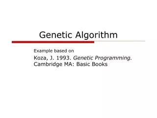
WTA – Example We define the Pk matrix for each weapon i and target j as the probability that weapon i will ‘kill’ target j if assigned to it Let the Pk matrix for our example be the following: Special Case: Suppose we find out that weapon 1 can only hit targets 2 and 3, while weapons 2 and 3 can hit all three targets Then the kill matrix is updated as follows .69 0 .03 .77 .32 .44 .80 Pk(i,j) = .95 .38 .19 We define the Pl array for each target j as the probability that target j will destroy the assets if it is able to leak through the weapon defenses • Let the Pl matrix for our example be the following: Pl(j) = .93 .17 .15
Comparison of Algorithms Heuristic Algorithms Exact Algorithm Greedy Algorithm Exhaustive Search Local Search Global Search MMR is fast, but also less accurate GA presents a tradeoff between MMR and BF, it finds an acceptably accurate solution in a reasonable time Speed Accuracy BF yields optimal solution, but is very slow
Heuristic Algorithms • Many different heuristic algorithms have been proposed • Genetic Algorithm • Simulated Annealing • Ant Colony Optimization • Branch and Bound Algorithms • Very Large-Scale Neighborhood • Stable Marriage Algorithm, etc. • No exact algorithms exist for solving the WTA in efficient time, so heuristic algorithms must be used • Pros and Cons to each Heuristic Algorithm • Solution strength based on comparison with other heuristic algorithms
Brute Force (BF) • Exhaustive search of the solution space • Not a computationally efficient algorithm • Enumerate all possible pairings to find optimal pairing Ex. Solutions are represented in array form where the position in the array represents the weapon and the value represents the target [1 1 1] [1 1 2] [1 1 3] [1 2 1] [1 2 2] [1 2 3] [1 3 1] [1 3 2] [1 3 3] [2 1 1] [2 1 2] [2 1 3] : C = .9188 [2 2 1] [2 2 2] [2 2 3] [2 3 1] [2 3 2] [2 3 3] [3 1 1] [3 1 2] [3 1 3] [3 2 1] [3 2 2] [3 2 3] [3 3 1] [3 3 2] [3 3 3] [1 1 1] : C = .3298 [1 1 2] : C = .4514 [1 1 3] : C = .4875 [1 2 1] : C = .2596 [1 2 2] : C = .4973 [1 2 3] : C = .5050 [1 3 1] : C = .2144 [1 3 2] : C = .4237 [1 3 3] : C = .4826 [2 1 1] : C = .3465 [2 1 2] : C = .8846 [2 1 3] : C = .9188 [2 2 1] : C = .2888 [2 2 2] : C = 1.1373 [2 2 3] : C = 1.1438 [2 3 1] : C = .2414 [2 3 2] : C = 1.0622 [2 3 3] : C = 1.1192 [3 1 1] : C = .2361 [3 1 2] : C = .7723 [3 1 3] : C = .8303 [3 2 1] : C = .1762 [3 2 2] : C = 1.0235 [3 2 3] : C = 1.0531 [3 3 1] : C = .2234 [3 3 2] : C = 1.0423 [3 3 3] : C = 1.1056 The array [2 1 3] represents the mapping of Weapon 1 to Target 2, Weapon 2 to Target 1 and Weapon 3 to Target 3 The cost C can be calculated as C = .93*(1-.69)0*(1-.32)1*(1-.95)0 + .17*(1-.03)1*(1-.44)0*(1-.38)0 + .15*(1-.77)0*(1-.80)0*(1-.19)1 = .9188 [1 1 1] : C = .3298 [1 1 2] : C = .4514 [1 1 3] : C = .4875 [1 2 1] : C = .2596 [1 2 2] : C = .4973 [1 2 3] : C = .5050 [1 3 1] : C = .2144 [1 3 2] : C = .4237 [1 3 3] : C = .4826 [2 1 1] : C = .3465 [2 1 2] : C = .8846 [2 1 3] : C = .9188 [2 2 1] : C = .2888 [2 2 2] : C = 1.1373 [2 2 3] : C = 1.1438 [2 3 1] : C = .2414 [2 3 2] : C = 1.0622 [2 3 3] : C = 1.1192 [3 1 1] : C = .2361 [3 1 2] : C = .7723 [3 1 3] : C = .8303 [3 2 1] : C = .1762 [3 2 2] : C = 1.0235 [3 2 3] : C = 1.0531 [3 3 1] : C = .2234 [3 3 2] : C = 1.0423 [3 3 3] : C = 1.1056
Maximum Marginal Return (MMR) • MMR is a greedy algorithm • Fast, but not as accurate as other methods* • At each iteration, select the weapon to target pair that yields the highest change in the cost function C Ex. Iteration 1: (Weapon-Target): ΔC 1-1: ΔC = .6417 1-2: ΔC = .0051 1-3: ΔC = .1155 2-1: ΔC = .2976 2-2: ΔC = .0748 2-3: ΔC = .1200 3-1: ΔC = .8835 3-2: ΔC = .0646 3-3: ΔC = .0285 Iteration 3: (Weapon-Target): ΔC 1-1: ΔC = .0321 1-2: ΔC = .0051 1-3: ΔC = .0231 Iteration 2: (Weapon-Target): ΔC 1-1: ΔC = .0321 1-2: ΔC = .0051 1-3: ΔC = .1155 2-1: ΔC = .0149 2-2: ΔC = .0748 2-3: ΔC = .1200 Iteration 2: (Weapon-Target): ΔC 1-1: ΔC = .0321 1-2: ΔC = .0051 1-3: ΔC = .1155 2-1: ΔC = .0149 2-2: ΔC = .0748 2-3: ΔC = .1200 Iteration 3: (Weapon-Target): ΔC 1-1: ΔC = .0321 1-2: ΔC = .0051 1-3: ΔC = .0231 Iteration 1: (Weapon-Target): ΔC 1-1: ΔC = .6417 1-2: ΔC = .0051 1-3: ΔC = .1155 2-1: ΔC = .2976 2-2: ΔC = .0748 2-3: ΔC = .1200 3-1: ΔC = .8835 3-2: ΔC = .0646 3-3: ΔC = .0285 Solution = [1 3 1] with cost C = .2144 Solution = [0 0 0] Solution = [0 0 1] Solution = [0 3 1] * For the special case where Pk(i, j) = Pk(i) or Pk(j) then MMR finds the optimal solution BF found solution [3 2 1] with C = .1762 The solution of 131 is NOT the optimal solution found by BF, in fact, it is second best
Genetic Algorithm (GA) • Developed by John Holland, University of Michigan (1970’s) • Based on Darwinian Natural Selection • Provides a combination of exploration (global search) and exploitation (local search) • Use crossover, mutation, eugenic operators to alter a population of chromosomes during each generation • Survival of the Fittest gives hope that the GA will converge to the optimal solution
Genetic Algorithm - Procedure • Initialization of Population • Evaluation of Population • Perform Genetic Operation • Crossover Operation • Eugenic Operation • Mutation Operation • Eugenic Operation • Evaluate all Chromosomes • Selection of Chromosomes
Genetic Algorithm - Initialization • Randomly assign weapon to target pairings for each chromosome to fill the population Ex. Let the population size = 5, then the population is randomly filled Pop1= [3 2 3] Pop2= [3 1 1] Pop3= [1 3 1] Pop4= [3 1 3] Pop5= [1 2 1] Terminology The array representation of the solution is referred to as the chromosome Each element in the chromosome is a gene
Genetic Algorithm - Evaluation • Evaluate the fitness of each chromosome • Probability of being a parent is defined as Ex. Pop1= [3 2 3] Pop2= [3 1 1] Pop3= [1 3 1] Pop4 = [3 1 3] Pop5= [1 2 1] Pop1= [3 2 3] Pop2= [3 1 1] Pop3= [1 3 1] Pop4= [3 1 3] Pop5= [1 2 1] C = 1.0531 C = .2361 C = .2144 C = .8303 C = .2596 Pparent = 0 Pparent = .3058 Pparent = .3139 Pparent = .0834 Pparent = .2970
Genetic Algorithm - Crossover • We use the Elite Preserving Crossover (GEX) Operator • Find genes with the same value i in both parents • Inherit “good” genes from both parents • Randomly select two genes not inherited • Exchange selected genes in both parents to generate offspring • Repeat for a specified number of crossovers Ex. For weapon 3, the Pk for each target is [.95, .38, .19] Thus the assignment of weapon 3 to target 1 yields the highest return, therefore this is a “good” gene A “good” gene is defined as a weapon-to-target pairing that yields the highest return among all target pairings with that weapon C1: [2 1 1] C2: [1 3 1] C1: [0 0 1] C2: [0 0 1] P1: [3 1 1] P2: [1 2 1]
Genetic Algorithm – Eugenic (1 of 2) • Eugenic process is used for local searches around the solutions • Create a temporary copy Plnew of Pl • For each target that has been assigned in the current chromosome, find Plnew x Pk for all weapons • Select weapon-to-target pairing that yields highest change in Plnew • Update Plnew • For each unassigned weapon, find Plnew x Pk for all targets • Select weapon-to-target pairing that yields highest change in Plnew • Update Plnew • Can be expressed as two stages of partial MMR • First stage allows new chromosome to inhabit characteristics of old chromosomes (examine assigned targets) • Second stage searches locally for better solution (examine unassigned targets)
Genetic Algorithm – Eugenic (2 of 2) C1: [2 1 1] C2: [1 3 1] E1 = [1 2 1] E1 = [0 0 0] E2 = [1 3 1] E1 = [0 0 1] E1 = [0 2 1] For C1, the assigned targets are Target 1 and Target 2 For Targets 1 and 2, the weapon-to-target pairing that yields the highest change in Plnew is Weapon 3 to Target 1 (.95 x .93 = .8835) Plnew is updated to [.8835 .17 .15] For Target 2, the weapon-to-target pairing that yields the highest change in Plnewis Weapon 2 to Target 2 (.44*.17 = .0748) Plnew is updated to [.8835 .0748 .15] Weapon 1 is unassigned, the weapon-to-target pairing that yields the highest change in Plnew is Weapon 1 to Target 1 (.69 X .8835 = .609615) Ex. W-T: ΔPlnew 1-1: ΔPlnew = .69 x .93 = .6417 1-2: ΔPlnew = .03 x .17 = .0051 2-1: ΔPlnew = .32 x .93 = .2976 2-2: ΔPlnew = .44 x .17 = .0748 3-1: ΔPlnew = .95 x .93 = .8835 3-2: ΔPlnew = .38 x .17 = .0646 W-T: ΔPlnew 1-2: ΔPlnew = .03 x .17 = .0051 2-2: ΔPlnew = .44 x .17 = .0748 3-2: ΔPlnew = .38 x .17 = .0646
Genetic Algorithm - Mutation • Mutation operator takes a chromosome and randomly changes a number of genes • Allows an exit of a local optimum in search of global optima Ex. C1 = [2 1 1] E1 = [1 2 1] Pop1 = [3 2 3] M1 = [2 1 3] M2 = [3 2 1] M3 = [3 3 3] ME1 = [2 3 1] ME2 = [2 3 1] ME3 = [1 3 1] After mutation operations are completed, the eugenic operator is applied to the newly mutated chromosomes
Genetic Algorithm - μ–λSelection • μ – λ Selection combines both old chromosomes and new ones • Delete redundant chromosomes • Select best remaining chromosomes • Refill population Ex. Pop1 = [3 2 3]: C = 1.0531 Pop2 = [3 1 1]: C = .2361 Pop3 = [1 3 1]: C = .2144 Pop4 = [3 1 3]: C = .8303 Pop5 = [1 2 1]: C = .2596 C1 = [2 1 1]: C = .3465 M1 = [2 1 3]: C = .9188 M2= [3 2 1]: C = .1762 M3 = [3 3 3]: C = 1.1056 ME1 = [2 3 1]: C = .2414 Pop1 = [3 2 3]: C = 1.0531 Pop2 = [3 1 1]: C = .2361 Pop3 = [1 3 1]: C = .2144 Pop4= [3 1 3]: C = .8303 Pop5 = [1 2 1]: C = .2596 C1 = [2 1 1]: C = .3465 C2 = [1 3 1]: C = .2144 E1= [1 2 1]: C = .2596 E2 = [1 3 1]: C = .2144 M1 = [2 1 3]: C = .9188 M2 = [3 2 1]: C = .1762 M3 = [3 3 3]: C = 1.1056 ME1= [2 3 1]: C = .2414 ME2 = [2 3 1]: C = .2414 ME3 = [1 3 1]: C = .2144 Pop1 = [3 2 3]: C = 1.0531 Pop2 = [3 1 1]: C = .2361 Pop3 = [1 3 1]: C = .2144 Pop4 = [3 1 3]: C = .8303 Pop5 = [1 2 1]: C = .2596 C1 = [2 1 1]: C = .3465 C2 = [1 3 1]: C = .2144 E1 = [1 2 1]: C = .2596 E2 = [1 3 1]: C = .2144 M1 = [2 1 3]: C = .9188 M2 = [3 2 1]: C = .1762 M3 = [3 3 3]: C = 1.1056 ME1 = [2 3 1]: C = .2414 ME2 = [2 3 1]: C = .2414 ME3 = [1 3 1]: C = .2144 Pop1 = [3 2 3]: C = 1.0531 Pop2 = [3 1 1]: C = .2361 Pop3 = [1 3 1]: C = .2144 Pop4 = [3 1 3]: C = .8303 Pop5 = [1 2 1]: C = .2596 C1 = [2 1 1]: C = .3465 M1 = [2 1 3]: C = .9188 M2 = [3 2 1]: C = .1762 M3= [3 3 3]: C = 1.1056 ME1 = [2 3 1]: C = .2414 Pop1 = [3 2 1]: C = .1762 Pop2 = [1 3 1]: C = .2144 Pop3 = [3 1 1]: C = .2361 Pop4= [2 3 1]: C = .2414 Pop5 = [1 2 1]: C = .2596 Repeat this procedure for however many generations are specified
Genetic Algorithm - Parameters • Simulations on several sets of data were run to find the optimal set of parameters with which to run the GA popSize – The population size nC – The number of crossovers nM – The number of mutations All data represented as ratio of parameter to max(W, T) We use the parameters that occur the most often in the quickest parameter sets • Best parameter set occurs when popSize = 1, nC = 5/3, nM = 5/2 of max(W, T) • Ex. If W = 5, T = 4, then popSize = 5, nC = 8, nM = 12
Results - Monte Carlo Simulation • For the case of W = 7 and T = 7, we were able to use Brute Force to find the optimal solution in a reasonable time • Monte Carlo simulation with 1000 trials yielded the following results The GA found the optimal solution in 952 of the 1000 trials, while the MMR algorithm only found the optimal solution 314 times The GA was slower than MMR but was still significantly faster than BF
Results - GA vs MMR GA Efficiency represents how much better the GA solution is than the MMR solution • Trends • GA Efficiency increases as W and T increases • GA Efficiency increases as W >> T • For cases where T > W, MMR is sufficiently close
Special Case Block Diagonal PkMatrix • We consider a special case where the Pk matrix is block diagonal • Consider the following scenario • Pk is the same for each weapon to target pairing for simplicity Weapons Targets 1 1 k 0 k 0 k k 0 0 0 0 k 0 k 0 k 2 2 2 2 Pk = 0 k k 0 k k 0 0 3 3 0 k 0 k 0 k 0 0 k 0 0 k 0 k 4 4 4 4 5 5 Note that if we can split Pk into n distinct groups, then we can split the problem into n subproblems
Results 5x5 and 7x7 Submatrices • For the case where W = 12 and T = 12, with submatrices of size 5x5 and 7x7, we found solutions using the following algorithms • MMR – MMR on the complete problem • MMR Partial – MMR on each of the subproblems, then combined • GA – GA on the complete problem • GA Partial – GA on each of the subproblems, then combined By splitting the problem into subproblems and using GA to solve both subproblems, we find a more optimal solution, as well as decreasing time significantly from the regular GA algorithm
Results 10x10 and 10x10 Submatrices • Similarly, we simulated a scenario where there were 20 weapons and 20 targets, with two groupings of 10 weapons and targets each
Conclusions • WTA problems are NP-Complete • GA can be used to find solutions to the WTA problem • GA’s are more accurate in finding solutions, however, MMR takes a much quicker time • When we can decompose the problem into smaller subproblems, this helps accuracy as well as time complexity • When the number of weapons outnumbers the number of targets, the GA is better than MMR
Future Work • Altering parameters for GA • Small nM at beginning, then larger towards later generations • Fuzzy logic controllers to find parameters • Extending the GA to the dynamic WTA problem • Hybrid algorithms • Use other algorithms for local searching • Relaxation of constraints • Semi-complete Pk or Pl matrices • Pk values not independent
Acknowledgments • Aaron Plotnik (38) and Dana Sinno (32) for their help and discussions on understanding the WTA problem • Sung-Hyun Son (32) for the numerous hours of supervision and guidance provided • Aneeb Qureshi (32) whose thoughtful musings provided many creative insights