Improve Phase Designing Experiments

1. Improve PhaseDesigning Experiments

2. Designing Experiments Welcome to Improve Process Modeling: Regression Advanced Process Modeling: MLR Reasons for Experiments Designing Experiments Graphical Analysis DOE Methodology Wrap Up & Action Items

3. Project Status Review • Understand our problem and its impact on the business. (Define) • Established firm objectives/goals for improvement. (Define) • Quantified our output characteristic. (Define) • Validated the measurement system for our output characteristic. (Measure) • Identified the process input variables in our process. (Measure) • Narrowed our input variables to the potential “X’s” through Statistical Analysis. (Analyze) • Selected the vital few X’s to optimize the output response(s). (Improve) • Quantified the relationship of the Y’s to the X’s with Y = f(x). (Improve)

4. Suppliers Inputs Define SIPOC VOC Project Scope P-Map, X-Y Matrix, FMEA, Capability Box Plot, Scatter Plots, Regression Fractional Factorial Full Factorial Center Points Customers Outputs Contractors Employees Measure (X1) (X11) (X9) (X8) (X3) (X2) (X4) (X7) (X10) (X6) (X5) (X11) (X3) (X1) (X4) Analyze (X8) (X5) (X2) (X5) (X3) Improve (X11) (X4) Business Success Control Plan Six Sigma Strategy

5. Reasons for Experiments • The Analyze Phase narrowed down the many inputs to a critical few now it is necessary to determine the proper settings for these few inputs because: • The vital few potentially have interactions. • The vital few will have preferred ranges to achieve optimal results. • Confirm cause and effect relationships among factors identified in Analyze Phase (e.g. Regression) • Understanding the reason for an experiment can help in selecting the design and focusing the efforts of an experiment. • Reasons for experimenting are: • Problem Solving (Improving a process response) • Optimizing (Highest yield or lowest customer complaints) • Robustness (Constant response time) • Screening (Further screening of the critical few to the vital few X’s) Design where you’re going - be sure you get there!

6. Desired Results of Experiments • Problem Solving • Eliminate defective products or services. • Reduce cycle time of handling transactional processes. • Optimizing • Mathematical model is desired tomove the process response. • Opportunity to meet differing customer requirements (specifications or VOC). • Robust Design • Provide consistent process or product performance. • Desensitize the output response(s) to input variable changes including NOISE variables. • Design processes knowing which input variables are difficult to maintain. • Screening • Past process data is limited or statistical conclusions • prevented good narrowing of critical factors in Analyze • Phase. When it rains it PORS!

7. DOE Models vs. Physical Models • What are the differences between DOE modeling and physical models? • A physical model is known by theory using concepts of physics, chemistry, biology, etc... • Physical models explain outside area of immediate project needs and include more variables than typical DOE models. • DOE describes only a small region of the experimental space. The objective is to minimize the response. The physical model is not important for our business objective. The DOE Model will focus in the region of interest.

8. Definition for Design of Experiments Design of Experiments (DOE) is a scientific method of planning and conducting an experiment that will yield the true cause and effect relationship between the X variables and the Y variables of interest. DOE allows the experimenter to study the effect of many input variables that may influence the product or process simultaneously, as well as possible interaction effects (for example synergistic effects). The end result of many experiments is to describe the results as a mathematical function. Y = f (x) The goal of DOE is to find a design that will produce the information required at a minimum cost. Properly designed DOE’s are more efficient experiments.

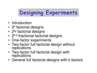
9. Yield Contours Are Unknown To Experimenter 75 80 135 85 6 Pressure (psi) 130 90 1 3 2 5 4 125 95 120 7 31 32 33 34 35 30 Temperature (C) One Factor at a Time is NOT a DOE One Factor at a Time (OFAT) is an experimental style but not a planned experiment or DOE. The graphic shows yield contours for a process that are unknown to the experimenter. Optimum identified with OFAT True Optimum available with DOE

10. Types of Experimental Designs • The most common types of DOE’s are: • Fractional Factorials • 4-15 input variables • Full Factorials • 2-5 input variables • Response Surface Methods (RSM) • 2-4 input variables ResponseSurface Full Factorial KNOWLEDGE Fractional Factorials

11. Nomenclature for Factorial Experiments • The general notation used to designate a full factorial design is given by: • Where k is the number of input variables or factors. • 2 is the number of “levels” that will be used for each factor. • Quantitative or qualitative factors can be used. 2k

12. (+1,+1) (-1,+1) 600 300 Temp 350 -1 -1 +1 22 Press +1 -1 -1 500 -1 +1 -1 Press 600 +1 +1 +1 500 (+1,-1) (-1,-1) Uncoded levels for factors 300F Temp 350F T P T*P Coded levels for factors Visualization of 2 Level Full Factorial • Four experimental runs: • Temp = 300, Press = 500 • Temp = 350, Press = 500 • Temp = 300, Press = 600 • Temp = 350, Press = 600

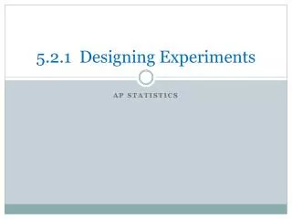
13. 8.2 4.55 A B C Response Run Start Stop Meters Number Angle Angle Fulcrum Traveled 1 -1 -1 -1 2.10 2 1 -1 -1 0.90 3 -1 1 -1 3.35 4 1 1 -1 1.50 5 -1 -1 1 5.15 6 1 -1 1 2.40 7 -1 1 1 8.20 8 1 1 1 4.55 3.35 1.5 5.15 2.4 Stop Angle Fulcrum Start Angle 2.1 0.9 Graphical DOE Analysis - The Cube Plot Consider a 23 design on a catapult... What are the inputs being manipulated in this design? How many runs are there in this experiment?

14. Graphical DOE Analysis - The Cube Plot • This graph is used by the experimenter to visualize how the response data is distributed across the experimental space. Stat>DOE>Factorial>Factorial Plots … Cube, select response and factors How do you read or interpret this plot? What are these? Catapult.mtw

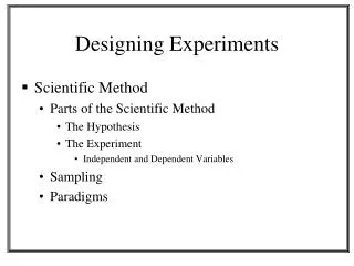
15. Graphical DOE Analysis - The Main Effects Plot • This graph is used to see the relative effect of each factor on the output response. Stat>DOE>Factorial>Factorial Plots … Main Effects, select response and factors Hint: Check the slope! Which factor has the largest impact on the output?

16. Main Effects Plot Creation Avg Distance at Low Setting of Start Angle: 2.10 + 3.35 + 5.15 + 8.20 = 18.8/4 = 4.70 Main Effects Plot (data means) for Distance -1 1 -1 1 -1 1 5.2 4.4 Dist 3.6 2.8 2.0 Start Angle Stop Angle Fulcrum Avg. distance at High Setting of Start Angle: 0.90 + 1.50 + 2.40 + 4.55 = 9.40/4 = 2.34 Run # Start Angle Stop Angle Fulcrum Distance 1-1-1-1 2.10 21-1-10.90 3-1 1-1 3.35 41 1-11.50 5-1-1 1 5.15 61-1 12.40 7-1 1 1 8.20 81 1 14.55

17. Higher B- Y Output B+ Lower - + A Interaction Definition When B changes from low to high the output drops dramatically. When B changes from low to high the output drops very little.

18. No Interaction SomeInteraction Full Reversal High High High B- B- B- B+ B+ Y Y B+ Y B+ Low Low Low - - - + + + A A A Strong Interaction Moderate Reversal High High B- B- Y Y B+ B+ B+ Low Low - - + + A A Degrees of Interaction Effect

19. Interaction Plot (data means) for Distance Start Angle 6.5 -1 1 5.5 4.5 Mean 3.5 2.5 1.5 -1 -1 1 1 Fulcrum Interaction Plot Creation (4.55 + 2.40)/2 = 3.48 (0.90 + 1.50)/2 = 1.20 Run # Start Angle Stop AngleFulcrumDistance 1-1-1-1 2.10 2 1-1-10.90 3-1 1-13.35 4 1 1-11.50 5-1-1 15.15 6 1-1 12.40 7-1 1 18.20 8 1 1 14.55

20. Graphical DOE Analysis - The Interaction Plots Stat>DOE>Factorial>Factorial Plots … Interactions, select response and factors When you select more than two variables MINITABTM generates an Interaction Plot Matrix which allows you to look at interactions simultaneously. The plot at the upper right shows the effects of Start Angle on Y at the two different levels of Fulcrum. The red line shows the effects of Fulcrum on Y when Start Angle is at its high level. The black line represents the effects of Fulcrum on Y when Start Angle is at its low level. Note: In setting up this graph we selected options and deselected “draw full interaction matrix”

21. Graphical DOE Analysis - The Interaction Plots Stat>DOE>Factorial>Factorial Plots … Interactions, select response and factors • The plots at the lower left in the graph below (outlined in blue) are the “mirror image” plots of those in the upper right. It is often useful to look at each interaction in both representations. Choose this option for the additional plots.

22. DOE Methodology • Define the Practical Problem • Establish the Experimental Objective • Select the Output (response) Variables • Select the Input (independent) Variables • Choose the Levels for the Input Variables • Select the Experimental Design • Execute the experiment and Collect Data • Analyze the data from the designed experiment and draw Statistical Conclusions • Draw Practical Solutions • Replicate or validate the experimental results • Implement Solutions

23. Generate Full Factorial Designs in MINITABTM “DOE”>”Factorial”>”Create Factorial Design…”

24. Create Three Factor Full Factorial Design Stat>DOE>Factorial>Create Factorial Design

25. Create Three Factor Full Factorial Design

26. Create Three Factor Full Factorial Design

27. Three Factor Full Factorial Design Hold on! Here we go….

28. At this point you should be able to: Determine the reason for experimenting Describe the difference between a physical model and a DOE model Explain an OFAT experiment and its primary weakness When shown a Main Effects Plots and interactions, determine which effects and interactions may be significant. Create a Full Factorial Design Summary