CS6234: Lecture 4
380 likes | 396 Views
This lecture covers linear programming, the simplex algorithm, duality, and the primal-dual algorithm in combinatorial optimization. It also discusses the formulation of LP problems in general and standard forms, as well as complementary slackness and the shortest path problem.

CS6234: Lecture 4
E N D
Presentation Transcript
CS6234: Lecture 4 • Linear Programming • LP and Simplex Algorithm [PS82]-Ch2 • Duality [PS82]-Ch3 • Primal-Dual Algorithm [PS82]-Ch5 • Additional topics: • Reading/Presentation by students Lecture notes adapted from Comb Opt course by Jorisk, Math Dept, Maashricht Univ,
Combinatorial Optimization Chapter 3 of [PS82] Duality Combinatorial Optimization Masters OR
LP in general form min c´ x s.t. a´i x = bi i ε M a´i x ≤ bi i ε M´xj ≥ 0 j ε N xjfree j ε N´ • Introduce surplus variables for inequality constraints • Replace free variables by two non-negative variables. Combinatorial Optimization Masters OR
In standard form… min c~´ x~ s.t. A~ x~ = b x~ ≥ 0 where A~ has extra columns for x´s in N´, and for slack variables, x~has extra variables for x´s in N´ and for slack variables, c~has extra elements for x´s in N´. Combinatorial Optimization Masters OR
Starting the dual The simplex method gives an optimal solution x0~ to the LP in standard form, with a basis Q, satisfying c~´– (cB~´B~-1)A~ ≥ 0. Thus, π´ = cB~´B~-1is a feasible solution to the problem π´ A~ ≤ c~´where πε Rm. Combinatorial Optimization Masters OR
The dual • π´ Aj≤ cj, for j ε N, • π´ Aj≤ cj, for j ε N´, andπ´ Aj≤ –cj, for j ε N´, and hence π´ Aj= cj, for j ε N´. • –πi≤ 0, for i ε M´, orπi≥ 0, for i ε M´. Objective: max π´ b. Combinatorial Optimization Masters OR
Definition of the Dual Definition 3.1: Given an LP in general form, called the primal, the dual is defined as follows Combinatorial Optimization Masters OR
Strong duality Theorem 3.1: If an LP has an optimal solution, so does its dual, and at optimality their costs are equal. Proof. Let x and π be optimal solutions to the primal and the dual resp., then c´x ≥ π´Ax ≥ π´b. (*) From the primal From the dual Combinatorial Optimization Masters OR
Strong duality proof Thus the primal has cost at least as high as the dual. Then, if the primal has a feasible solution, the cost of the dual cannot be unbounded. It has feasible solution π´, and since it is not unbounded, it must have an optimum. The cost of π´ is π´b = cB~´B~-1 b = cB~´x0~ which is the optimal solution of the primal. Together with (*) this suffices to prove the Theorem. Combinatorial Optimization Masters OR
The dual of the dual Theorem 3.2. The dual of the dual is the primal. Proof. Left as an exercise. Theorem 3.3: Given a primal-dual pair, either of the following holds: • Both have a finite optimum • Both are infeasible • One is unbounded the other is infeasible Proof. Skip. Combinatorial Optimization Masters OR
Complementary slackness Theorem 3.4: A pair, x, π, respectively feasible in a primal-dual pair is optimal if and only if: ui = πi(a´i x - bi) = 0 for all i (1) vj = (cj - π´Aj)xj= 0 for all j. (2) Combinatorial Optimization Masters OR
Complementary slackness (2) Proof:Recall ui=πi(a´i x - bi) & vj=(cj- π´Aj)xj Define u = ui (≥ 0) & v = vj (≥ 0) Thus, u =0 if and only if (1) holds (each ui=0) and v = 0 if and only if (2) holds (each vj=0). Now, notice that (u + v) = c´x – π´b. Thus, if (1) and (2) hold, (u + v) = 0, and c´x = π´b. This implies that x and π have the same objective value, and hence are both optimal. Combinatorial Optimization Masters OR
Complementary slackness (3) Consequences: If an inequality constraint in the dual is not binding, then the corresponding primal variable must have value zero and vice versa. Likewise, if a nonnegative variable has strictly positive value, then the corresponding constraint must be binding. Combinatorial Optimization Masters OR
Tableau (for example 2.6) Min Z = x1 + x2 + x3 + x4 + x5 s.t. 3x1 + 2x2 + x3 = 1 5x1 + 2x2 + x3 + x4 = 3 2 x1 + 5 x2 + x3 + x5 = 4 Combinatorial Optimization Masters OR
Simplex Algorithm (Tableau Form) Diagonalize to get bfs { x3, x4, x5 } Determine reduced cost by making c~j = 0 for all basic col Combinatorial Optimization Masters OR
Combinatorial Optimization Masters OR
Farkas Lemma Skip 3.3 Combinatorial Optimization Masters OR
The shortest path problem and its dual Definition 3.3 Given a directed graph G=(V,E) and a nonnegative weight cj ≥ 0 associated with each arc ejε E, an instance of the shortest path problem (SP) is the problem of finding a directed path from a distinguished source node s to a distinguished terminal node t, with the minimum total weight. Combinatorial Optimization Masters OR
Shortest path problem Feasible set F is given by F = {P = (ej1,..,ejk) : P is a directed path from s to t in G}. Cost c(P) = Σi=1k cji . Formulation as LP uses node-arc incidence matrix A: 1 if arc j leaves node i aij = { -1 -f arc j enters node i 0 otherwise Combinatorial Optimization Masters OR
a e1 3 1 e4 2 s t e3 e5 2 1 e2 b SP Example Combinatorial Optimization Masters OR
LP formulation Min e1+ 2e2+ 2e3 + 3e4 + e5 s.t. e1 +e2= 1 - e4 - e5 = -1 - e1 e3 + e4 = 0 - e2 - e3 + e5 = 0 0 ≤ ei ≤ 1, i =1…5 Combinatorial Optimization Masters OR
Redundancy Claim: Any solution that satisfies 3 of the four constraints, satisfies all 4 of them. Easily checked. Thus, we omit the constraint for the sink t. Next, we consider the tableau of a feasible solution Combinatorial Optimization Masters OR
a e1 3 1 e4 2 s t e3 e5 2 1 e2 b Starting Tableau Combinatorial Optimization Masters OR
Summary of LP for SP • Simplex algorithm in tableau form • Cost vector c is also included as a constraint (Read details in [PS82]-Ch-2) • Each basis has (n-1) edges; • Not all are positive; • Edges with +ve flows are on the (s-t) path • Pivoting – bring in a new edge; • Based on relative cost (row0 of tableau) Clever idea! Combinatorial Optimization Masters OR
a e1 3 1 e4 2 s t e3 e5 2 1 e2 b Starting Tableau To prepare basis { e1, e4, e5 }: row2 row2 + row1; Combinatorial Optimization Masters OR
a e1 3 1 e4 2 s t e3 e5 2 1 e2 b Initial feasible bfs (1) After we have row-2 row-1 + row-2; Basis { e1, e4, e5 }: e1=1, e4=1, e5 =0, this bfs is degenerate Now, to adjust reduced costs; First, row-0 row-0 - row-1 Combinatorial Optimization Masters OR
a e1 3 1 e4 2 s t e3 e5 2 1 e2 b Initial feasible bfs (2) After we have row 2 row 1 + row 2; After, row 0 row 0 - row 1; Then, row-0 row-0 – 3*(row-2); Combinatorial Optimization Masters OR
a e1 3 1 e4 2 s t e3 e5 2 1 e2 b Initial feasible bfs (3) After we have row 2 row 1 + row 2; Then, row 0 row 0 + row 1; Then, row 0 row 0 – 3*(row 2); Then, row-0 row-0 – row-3; Combinatorial Optimization Masters OR
a e1 3 1 e4 2 s t e3 e5 2 1 e2 b Initial feasible bfs (4) After we have row 2 row 1 + row 2; Then, row 0 row 0 + row 1; Then, row 0 row 0 – 3*(row 2);Then, row 0 row 0 + *(row 3) Basis { e1, e4, e5 }: e1=1, e4=1, e5 =0, this bfs is degenerate Combinatorial Optimization Masters OR
a e1 3 1 e4 2 s t e3 e5 2 1 e2 b Pivoting (1) Choose col with -ve relative-cost; (bring col e2 into the basis) Choose pivot from that column; Now, perform: (a) row1 row1 – row2; (b) row3 row3 + row1; Combinatorial Optimization Masters OR
a e1 3 1 e4 2 s t e3 e5 2 1 e2 b Pivoting (2) Now, to bring e2 into the basis; After (a) and (b); Now, get reduced cost: (c) row0 row0 + row2; Combinatorial Optimization Masters OR
a e1 3 1 e4 2 s t e3 e5 2 1 e2 b Pivoting (3) Now, to bring e2 into the basis; After (a) and (b); And (c); This solution is optimal. All relative cost (row0) are positive! Combinatorial Optimization Masters OR
a e1 3 1 e4 2 s t e3 e5 2 1 e2 b The dual of SP Max πs – πt s.t. π´A ≤ c´. πfree. In case of SP: the constraints of the dual are: πi – πj ≤ cij. Combinatorial Optimization Masters OR
Complementary slackness for SP A path f as defined by primal variables, and an assignment of dual variables πare jointly optimal if and only if: • A primal variable with positive value corresponds to a dual constraint that is satisfied at equality. • A dual constraint not satisfied at equality corresponds to a primal variable with value zero. Combinatorial Optimization Masters OR
a a e1 e1 3 3 1 1 e4 e4 2 2 s s t t e3 e3 e5 e5 2 2 1 1 e2 e2 b b ? 0 3 1 Min e1 + 2e2 + 2e3 + 3e4 + e5 s.t. e1 +e2 = 1 - e4 -e5 = -1 - e1 + e3 + e4 = 0 - e2 - e3 + e5 = 0 0 ≤ ei ≤ 1, for i =1…5 Min πs – πt s.t. πs - πa 1 πs - πb 2 πa - πb 2 πa - πt 3 πb - πt 1 each πi 0 Compare dual variables πwith label used in Dijkstra algorithm for shortest path! Combinatorial Optimization Masters OR
Read up the following sectionson your own. Sect 3.5: Dual Info in the Tableau Sect 3.6: Dual Simplex Algorithm Sect 3.7: Intrepretation of Dual Simplex Algorithm Combinatorial Optimization Masters OR
Some Suggested Exercises: All from [PS82] • Theorem 3.3 • 3 • 11 • 12 • 13 • 17 Combinatorial Optimization Masters OR
Thankyou. Q & A