Balanced Binary Search Trees

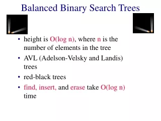
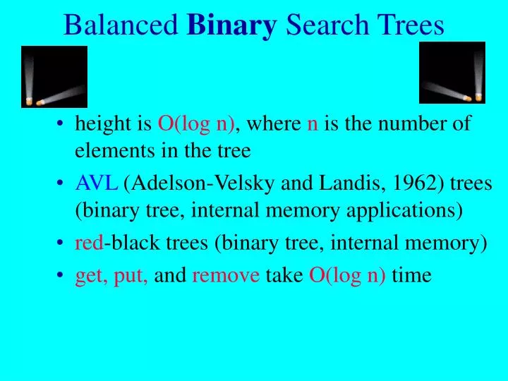
Balanced Binary Search Trees height is O(log n), where n is the number of elements in the tree AVL (Adelson-Velsky and Landis, 1962) trees (binary tree, internal memory applications) red-black trees (binary tree, internal memory) get, put, and remove take O(log n) time

Balanced Binary Search Trees Indexed AVL trees Indexed red-black trees Indexed operations alsotakeO(log n) time

Balanced Search Trees weight balanced binary search trees B-tree degree > 2, external memory applications (eg DB) 2-3 trees etc.

Dictionary Structures

Hashing • In practice hashing will outperform balanced search trees for search, insert, delete. • Balanced search trees used only when must guarantee a worst case time. • Balanced ST used when search and delete done by rank. • Balanced ST used when operations are not done by exact key match (eg, find smallest element with key larger than k).

Comparing Search Trees • Run-time performance of AVL and red-black trees similar. • Splay trees take less time to perform a sequence of u operations. • Splay trees easier to implement.

Comparing Search Trees • AVL and red-black trees use “rotations” to maintain balance. • AVL perform 1 rotation after an insert and O(log n) rotations after a delete. • red-black trees perform a single rotation following either an insert or delete. • In most applications a rotation takes Q(1) time so difference is not important. • In advanced applications rotations cannot be performed in constant time. • Example: balanced priority search trees of McCreight. Represent 2D arrays. Each rotation costs O(log n). • RBT: insert/delete remain at O(log n). • AVL: insert O(log n) but delete is O(log2n).

Comparing Search Trees • AVL, red-black, splay trees good when dictionary can fit into main memory. • B-tree good when dictionary is so large that it must be kept on disk. • In this case want high degree and smaller height.

Implementation • Some Java code available on web site (as solution to exercises). • The classes java.util.TreeMap and java.util.TreeSet use red-black trees. • Applications of balanced trees same as for BST from last chapter.

AVL Tree • binary tree, created in 1962 by Adelson-Velskii and Landis • Definition: • An empty binary tree is an AVL tree • If T is a nonempty binary tree with TL and TR as its left and right subtrees, then T is an AVL tree iff • TL and TR are AVL trees and • |hL - hR| <= 1 where hL and hR are the heights of TL and TR respectively.

AVL Tree • An AVL search Tree is a binary search tree that is also an AVL tree. • An indexed AVL search tree is an indexed binary search tree that is also an AVL tree. • do not cover in this chapter • same techniques carry over to iAVL trees

AVL Tree a and b are AVL trees. c is not (height wrong). a is NOT an AVL search tree (not a search tree) b is an AVL search tree.

AVL Tree Both trees are AVL search trees.

AVL Tree Both trees are indexed AVL search trees.

AVL TreeProperties, part 1 • The height of an AVL tree with n elements is O(log n) • For every value of n, n>=0, there exists an AVL tree (otherwise some insertions cannot create an AVL tree). • An n-element AVL search tree can be searched in O(height) = O(log n)

AVL TreeProperties, part 2 • A new element can be inserted into an n-element AVL search tree so that the result is an n + 1 element AVL tree and can be done in O(log n) time. • An element can be deleted from an n-element AVL search tree, n > 0, so that the result is an n - 1 element AVL tree and can be done in O(log n) time.

Height The height of an AVL tree that has n nodes is at most 1.44 log2 (n+2). The height of every n node binary tree is at least log2 (n+1).

Height The height of an AVL tree that has n nodes is at most 1.44log2 (n+2). Proof: Let Nh be the minimum number of nodes in an AVL tree of height h. worst case: height of on of the subtrees is h-1 and height of the other is h-2. Both are AVL trees. Hence: Nh = Nh-1+Nh-2 + 1, N0=0, N1=1. Similar to the definitoin of the Fibonacci numbers: Fn=Fn-1+Fn-2, F0=0, F1=1

Height The height of an AVL tree that has n nodes is at most 1.44 log2 (n+2). Proof (continued): can show: Nh =Fh+2-1 for h >=0. From Fibonacci number theory, know that Fh so if there are n nodes in the tree then h is at most

AVL Tree • for every node x, define its balance factor balance factor of x = height of left subtree of x - height of right subtree of x • balance factor of every node x is -1, 0, or 1

Balance Factors -1 1 1 -1 0 1 This is an AVL tree. 0 0 -1 0 0 0 0

-1 10 1 1 7 40 -1 0 1 0 45 3 8 30 0 -1 0 0 0 60 35 1 20 5 0 25 AVL Search Tree

AVL Search Tree • Searching. Use same code as for binary search tree. • Since height of an AVL tree with n elements is O(log n), search time is O(log n) • Inserting: if use same code as for binary search tree, resulting tree may not be an AVL tree.

AVL Search Tree • Example: insert 32 into figure Resulting tree is unbalanced (left figure). Can restore balance by shifting subtrees (right figure).

AVL serach treeinserting: observations • O1: In the unbalanced tree the balance factors are limited to -2, -1, 0, 1, and 2 • O2: A node with balance factor 2 had a balance factor 1 before the insertion. A node with balance factor -2 had a balance factor -1 before the insertion.

AVL serach treeinserting: observations • O3: The balance factors of only those nodes on the path from the root to the newly inserted node can change as a result of the insertion. • O4: Let A denote the nearest ancestor of the newly inserted node whose balance factor is either -2 or 2 (in previous example, the node A would be node 40). The balance factor of all nodes on the path from A to the newly inserted node was 0 prior to the insertion.

AVL serach treeinserting: observations on node A • Node A may be identified while we are moving down from the root searching for the place to insert the new element. • From O2, bf(A) was either 1 or -1 prior to the insertion. • Let X denote the last node encountered that has bf 1 or -1.

AVL serach treeinserting: observations on node X • Examples: if insert 32 into below AVL tree, X is 40: If insert 22, 28, 50 into below tree, X is node 25

AVL serach treeinserting: observations on node X • When node X does not exist, all nodes on path from root to new node have balance factor 0 prior to insertion. • Thus tree cannot be unbalanced since insertion changes balance factors by -1, 0, or 1 and only bf on path to new node can be changed.

AVL serach treeinserting: observations on node X • If bf (X) = 0 after insertion, then the height of the subtree with X as root is the same before and after the insertion. • Example: • if subtree rooted at X had height h before insertion and if bf(X) was 1, • then the height of its left subtree XL was h-1 • and the height of its right subtree XR was h-2

AVL serach treeinserting: observations on node X • Example continued: • For balance factor to become 0, insertion must be made in XR resulting in X’R of height h-1 • height of X’R must increase to h-1 as all balance factors on path from X to new node were 0 prior to insertion. • height of X remains h, and balance factors of the ancestors of X are same before and after insertion, so tree is balanced.

AVL serach treeinserting: observations on node X • Example continued: • Only way tree can become unbalanced is if insertion causes bf(X) to change from -1 to -2 or 1 to 2. • For latter to occur, insertion must be made in left subtree XL of X. • Now height of X’L must become h because all balance factors • on path from X to new node were 0 prior to insertion. • Thus X is the node A referred to in O4.

AVL serach treeinserting: classifying imbalances • Two main classes: • L new node is in left subtree of A • R new node is in right subtree of A • Can refine: • LL: the left grandchild of A is on the path to new node. • Such a grandchild exists as the height of subtree of A that contains the new node must be at least 2 for the bf(A) to be -2 or 2. • LR: the right grandchild of A is on path to new node. • RR: symmetrical situation to LR • RL : symmetrical situation to LL

LL imbalance • Rotation: • bf(B) = 0, otherwise B would have been designated as the node A. • Node B becomes the root the subtree that A was previously root of. • B’L remains the left subtree of B. • A becomes the root of B’s right subtree • BR becomes left subtree of A • right subtree of A is unchanged.

LL imbalance continued • Balance result: • Balance factors of nodes in B’L that are on the path from B to new node change • Balance factor of A changes • Remaining balance factors are same as before the rotation. • Heights of figures a and c below are same so balance factors of their ancestors are the same. • Thus a single LL rotation at A rebalances the entire tree.

LR imbalance • Rotation: • Node C becomes the root of the subtree that A was previously root of. • BL remains the left subtree of B. • A becomes the root of C’s right subtree • CR becomes left subtree of A (if it exists) • CL becomes right subtree of B (if it exists) • right subtree AR of A is unchanged.

LR imbalance continued • Balance result: • Balance factors of nodes B and A following the rearrangement depend on the value b of bf( C) just after the insertion but before the rearrangement. • Heights of figures a and c below are same so balance factors of their ancestors are the same. • Thus a single LR rotation at A rebalances the entire tree.

AVL rotations • RR and RL rotations are symmetric to LL and LR. • LL and RR imbalances called single rotations. • LR and RL imbalances are called double rotations. • A LR transformation can be viewed as an RR rotations followed by an LL rotation. • A RL transformation can be viewed as a LL rotation followed by an RR rotation.

AVL rotations

put(9) -1 10 0 1 1 7 40 -1 0 1 -1 0 45 3 8 30 0 -1 0 0 0 0 60 35 1 9 20 5 0 25

put(29) -1 10 1 1 7 40 -1 0 1 0 45 3 8 30 0 -1 0 0 0 -2 60 35 1 20 5 0 -1 RR imbalance => new node is in right subtree of right subtree of blue node (node with bf = -2) 25 0 29

RR rotation 1 2 0 A A B 0 -1 0 AL 0 B AL B B’R A h h h+1 h+1 BL BR BL B’R AL BL h h h h+1 h h before insertion after inserting into BR after RR rotation RR imbalance => new node is in right subtree of right subtree of node (node with bf = -2)

RR rotation See web site.

put(29) -1 10 1 1 7 40 -1 0 1 0 45 3 8 30 0 0 0 0 0 60 35 1 25 5 0 0 20 29 RR rotation.

put(27) LR imbalance => new node is in right subtree of left subtree of blue node (node with bf = 2) -1 10 1 1 7 40 -1 0 2 0 45 3 8 30 0 -1 0 0 60 0 35 1 25 5 0 1 20 29 0 Node C from next slide is 29 so bf( C)= 1 27

LR rotation after inserting into BR 2 1 0 A A C -1 0 B AR AR B A B h h C BL BR BL b BL CL h h h CR AR h h before insertion after RR rotation CL CR b = 0 => bf(B)=bf(A)=0 after rotation b = 1 => bf(B)=0 bf(A)= -1 after rotation b = -1 => bf(B)=1 bf(A)=0 after rotation Node C from previous slide is 29 so bf( C)= 1 => bf(B)=0 bf(A)= -1

put(27) Node C was node 29 Node B was node 25 Node A was node 30 -1 10 1 1 7 40 -1 0 0 0 45 29 3 8 0 0 -1 0 0 60 1 25 30 5 0 0 0 20 27 35 bf(B)=0 bf(A)= -1 as predicted on previous slide

AVL trees deletion • Delete as from a BST • Let q be the parent of the node that was physically deleted. divert 20’s right pointer to 30 and then q is 20 delete 25 so q is old node 15 (new node 12) delete 15 its node is used by 12 node 12 is physically deleted

AVL trees deletion • Delete as from a BST • Let q be the parent of the node that was physically deleted. delete 15 its node is used by 14 soqis node 13 (parent of old node 14) 13 10 node 14 is physically deleted 14

AVL trees deletion • Balance factors of some or all of the nodes on the path from the root to q change as result of deletion. • Must retrace this path backward from q toward root. • If deletion took place from the left subtree of q then bf(q) decreases by 1. • If deletion took place from right subtree of q then bf(q) increases by 1.

Balanced Binary Search Trees