Download
1 / 55
560 likes | 714 Views
Spanning Trees in Communication Networks. Rui Campos INESC Porto, Faculdade de Engenharia, Universidade do Porto rcampos@inescporto.pt. Outline. Graph Theory Spanning Trees Algorithms Spanning Trees Applications Summary. About me. PhD student at University of Porto PhD Overview

E N D
Spanning Trees in Communication Networks Rui Campos INESC Porto, Faculdade de Engenharia, Universidade do Porto rcampos@inescporto.pt
Outline • Graph Theory • Spanning Trees • Algorithms • Spanning Trees Applications • Summary
About me • PhD student at University of Porto PhD Overview Auto-configuration and Self-management of Personal Area Networks considering: • intra- and extra-PAN connectivity • heterogeneity in IP networks • integration of multiple communication technologies • Researcher at INESC Porto Participation in FP6 Ambient Networks Project • 1st phase - protocol design, specification, and simulation • 2nd phase – automatic and dynamic IP connectivity establishment between Ambient Networks
1. Graph Theory Graph formal definition: A graph G=(V,E,w) is defined as a set of verticesV connected by a set of edges E=[V]2(i.e., the elements of E are 2-element subsets of V) with weights wthat represent costs assigned to the edges of G.
1. Graph Theory [some definitions] • Number of vertices in G is n = |V| • Number of edges in G is m = |E| • Degree of a vertex vis defined as its number of adjacent edges (an adjacent edge to v is an edge connecting it to a neighbor vertex) • Path in Gis defined as a sequence of connected adjacent vertices • Cost of path is equal to sum of weights of edges belonging to path • Cycle in Gis defined as a path where first and last vertex in sequence are the same
1. Graph Theory [graph types] undirected undirected weighted
1. Graph Theory [graph types] directed directed weighted
1. Graph Theory [specific types] complete graph metric graph all vertices have degree n-1 edge weights satisfy triangle inequality
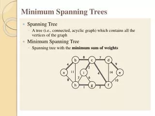
1. Graph Theory [specific types] tree spanning tree tree with n-1edges extracted from a graph G with n vertices graph without cycles
2. Spanning Trees [cost functions] • Path cost e.g., cT(1,3)=5+2=7 • Total cost Ctotal(T)=5+2+1=8 • Routing Cost Cr(T)= cT(1,2)+cT(1,3)+cT(1,4)+cT(2,1)+cT(2,3)+cT(2,4) + cT(3,1)+cT(3,2)+cT(3,4)+cT(4,1)+cT(4,2)+cT(4,3)=48
2. Spanning Trees [types] Shortest Path Tree (SPT) Minimum Spanning Tree (MST) Minimum Routing Cost Tree (MRCT) path cost total cost routing cost
2. Spanning Trees [SPT] The Shortest Path Tree (SPT) rooted at a vertex s defines a tree composed by union of the shortest paths between s and each of the other vertices in G such that:
2. Spanning Trees [SPT] Let’s see an example … SPT root at vertex 1: P(1,2) = (1,2) ; C(1,2) = 10 P*(1,2) = (1,3,2) ; C*(1,2) = 3 P**(1,2) = (1,3,4,2) ; C**(1,2) = 9 P(1,4) = (1,2,4) ; C(1,4) = 14 P*(1,4) = (1,2,3,4) ; C*(1,4) = 14 P**(1,4) = (1,3,2,4) ; C**(1,2) = 7 P***(1,4) = (1,3,4) ; C***(1,4) = 5 P(1,3) = (1,3) ; C(1,3) = 2 P*(1,3) = (1,2,3) ; C*(1,3) = 11 P**(1,3) = (1,2,4,3) ; C**(1,3) = 17
2. Spanning Trees [SPT] SPT root at vertex 1: P*(1,2) = (1,3,2) P(1,3) = (1,3) P***(1,4) = (1,3,4)
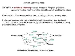
2. Spanning Trees[MST] The Minimum Spanning Tree (MST) represents the spanning tree T* such that: for all spanning trees T that can be computed from G
2. Spanning Trees[MST] Let’s see an example ... STs that can be computed from graph: Ctotal = 3+2+4 = 9 Ctotal = 3+5+4 = 12 Ctotal = 2+3+5 = 11 Ctotal = 2+4+5 = 11
2. Spanning Trees[MRCT] The Minimum Routing Cost Tree (MRCT) represents the spanning tree T* such that: for all spanning trees T that can be computed from G Note: computation of exact MRCT is a NP-hard problem
2. Spanning Trees [MRCT] Let’s see an example … STs that can be computed from graph: Cr = 12+4+9+12+8+3 +4+8+5+9+3+5=82 Cr = 2+4+5+2+6+3 +4+6+9+5+3+9=58 Cr = 2+4+9+2+6+11 +4+6+5+9+11+5=74 Cr = 2+10+5+2+8+3 +10+8+5+5+3+5=66
2. Spanning Trees [MRCT] Using other routing cost definition … STs that can be computed from graph: Cr = 12+4+9+8+3+5=41 Cr = 2+4+5+6+3+9=29 Cr = 2+4+9+6+11+5=37 Cr = 2+10+5+8+3+5=33
2. Spanning Trees[other types] • MRCT considering communication requirement (MRCT is optimal when communication requirements are equal) • Steiner Minimal Tree (SMT) • spans only a given subset of vertices in a graph G • minimizes same cost functions as MST • Minimum Diameter Spanning Tree (MDST) • diameter = cost of longest path between any two vertices in a tree • defines spanning tree of minimum diameter among all possible spanning trees Note: other types and further details can be found in [1]
2. Spanning Trees[2 interesting cases] • When edge weights of G are highly heterogeneous MST = MRCT = SPT (*) • When there is a single source s MRCT = SPTs (*) P. Mieghem, S. Langen, Influence of the link weight structure on the shortest path, Physical Review E 71 (2005) 056113-1–056113-13. P. Mieghem, S. M. Magdalena, Phase transition in the link weight structure of networks, Physical Review E 72 (2005) 056138-2–056138-7.
2. Spanning Trees[MST=MRCT=SPT] Let’s see an example ... STs that can be computed from graph: Cr=64; Ctotal=21 Cr=46; Ctotal=21 Cr=46; Ctotal=21 Cr=64; Ctotal =21 Cr=36; Ctotal =12 Cr=36; Ctotal =12 Cr=10; Ctotal =3 Cr=64; Ctotal =21 SPT
3. Algorithms[Prim’s algorithm] • Algorithm to compute MST for a graph G • Proposed by Robert Prim in 1957 • Time complexity O(n.m) • in its more naive implementation O(m.log(n)) • using binary heaps in conjunction with adjacency lists O(m+n.log(n)) • using Fibonacci heaps in conjunction with adjacency lists
Algorithm: PRIM Input: A weighted, undirected graph G=(V,E,w) Output: A minimum spanning tree T T ← 0 Let uV be an arbitrary vertex U ← {u} while |U| < n do find uU and v(V - U) such that edge (u,v) is the smallest edge between U and V – U and does not form a cycle T ← T {(u,v)} U← U {v}
3. Algorithms[Prim’s algorithm] Steps in a nutshell: (T ← 0) • Pick up arbitrary vertex v • Select edge (i,j) adjacent to v with lowest weight and add it to T • Select adjacent edge (i,j) to T with lowest weight that does not form a cycle and add it to T • Repeat step 3 until all vertices have been spanned
3. Algorithms[Prim’s algorithm] Let’s see an example ... input graph MST
3. Algorithms[Prim’s algorithm] Other possible result ... input graph MST
3. Algorithms[Kruskal’s algorithm] • Algorithm to compute MST for a graph G • Proposed by Joseph Kruskal in 1956 • Time complexity • O(m.log(m)) • using priority queues
Algorithm: KRUSKAL Input: A weighted, undirected graph G=(V,E,w) Output: A minimum spanning tree T Sort edges in E in nondecreasing order by weight T ← 0 Create one set for each vertex for each edge (u,v) in sorted order do if FIND_SET(u) FIND_SET(v) then T ←T {(u,v)} UNION(u,v) Legend
3. Algorithms[Kruskal’s algorithm] Steps in a nutshell: (T ← 0) • Pick up edge (i,j) with lowest weight that does not belong to T and does not form a cycle • Add edge (i,j) to T • Repeat step 1 and 2 until all vertices have been spanned
3. Algorithms[Kruskal’s algorithm] Let’s see an example ... input graph MST
3. Algorithms[Dijkstra’s algorithm] • Algorithm to compute SPT for a graph G • Proposed by Edsger Dijkstra in 1959 • Time complexity • O(n2) • in its more naive implementation • O(m.log(n)) • using binary heaps • O(m+nlog(n)) • using Fibonacci heaps
Algorithm: DIJKSTRA Input: A weighted, directed graph G=(V,E,w); a source vertex s. Output: A shortest path tree T rooted at s for each vV do δv ← ; pv ← NIL δs ← 0; T← 0; S ← V whileS 0 do choose uS with min(δu) S← S – {u} if u s then T← T {(pu,u)} for each vertex v adjacent to u do if (δv δu + w(u,v)) then δv ← δu + w(u,v) pv ← u
3. Algorithms[Dijkstra’s algorithm] Steps in a nutshell: (T ← 0; δv ← ; δs ← 0) • Select vertex v with min shortest path estimate and add edge (pv,v) to T • Re-evaluate shortest path estimates of vertices adjacent to v and update them and parent vertex in T if lower estimates are obtained • Repeat steps 1 and 2 until all vertices have been spanned
3. Algorithms[Dijkstra’s algorithm] Let’s see an example ... SPT rooted@vertex 1 input graph
3. Algorithms [Bellman-Ford algorithm] • Algorithm to compute SPT for a graph G • Proposed by Richard Bellman in 1958 • Works in more general cases • finds SPT even when graph has negative weights • Time complexity • O(n.m)
Algorithm: BELLMAN-FORD Input: A weighted, directed graph G=(V,E,w); a source vertex s. Output: A shortest path tree T rooted at s for each vV do δv ← ; pv ← NIL δs ← 0 for i ←1 to n-1 do for each (u,v)E do if (δv δu + w(u,v)) then δv ← δu + w(u,v); pv ← u for each (u,v)Edo if (δv δu + w(u,v)) then Output “A negative cycle exists”; Exit T← 0 forv(V-s) do T← T {(pu,u)}
3. Algorithms [Bellman-Ford algorithm] Steps in a nutshell: (T ← 0; δv ← ; δs ← 0) • For each edge (u,v) re-evaluate shortest path estimate δv and update it and pv if (δu + w(u,v) δv) • Repeat step 1 (n-1) times • The union of edges (pv,v) gives shortest path tree T
3. Algorithms [Bellman-Ford algorithm] Let’s see an example ... SPT rooted@vertex 2 E={(1,2),(2,1),(1,3),(3,1),(2,4),(4,3)} input graph Re-evaluation: for each (u,v)E do if (δu+ w(u,v) δv) then δv←δu+ w(u,v) SPT_rooted@2
3. Algorithms [Add algorithm] • Algorithm for finding approximate MRCT for a graph G • Proposed by Vic Grout in 2005 • Vertex oriented version of Prim’s algorithm • minimizes number of relay nodes in final spanning tree • Time complexity • O(n.log(n)) time in the worst case • usually, faster due to tendency for many nodes to be added to T at each step
Algorithm: ADD Input: undirected graph G=(V,E) Output: approximate minimum routing cost tree T T← 0 for allv V sv←0 for all u,v V wuv ←0 find u such that du ←max(dv), v V su←1 while there existsj such that sj = 0 do for each v V adjacent to u do wuv←1; sv←1; T← T {(pu,u)} find u such that (du− δu)← max(dj − δj) where sj = 1 Legend: sv=1 vT wuv – weight of edge (u,v) du – degree of vertex u δu – degree of vertex u in T
3. Algorithms [Add algorithm] Steps in a nutshell: • Pick up vertex v adjacent to maximum number of unspanned vertices • Add to T all edges adjacent to v that do not form a cycle • Repeat steps 1 and 2 until all vertices are added to T
3. Algorithms [Add algorithm] Let’s see an example ... approximate MRCT input graph
3. Algorithms [Wong’s algorithm] • Proposed by Richard Wong in 1980 • 2-approximate MRCT algorithm • Based on Dijkstra’s algorithm • Time complexity • O(n2.log(n)+m.n)
3. Algorithms [Wong’s algorithm] Steps: • Compute n SPTs using Dijkstra’s algorithm • Compute routing cost for each SPT • Select SPT with lowest routing cost 2-approximate MRCT
3. Algorithms [Wong’s algorithm] Let’s see an example ... SPT_rooted@3 SPT_rooted@1 SPT_rooted@2 SPT_rooted@8 SPT_rooted@6 SPT_rooted@4 SPT_rooted@5 SPT_rooted@7
3. Algorithms [Wong’s algorithm] Let’s see an example ... approximate MRCT
4. Spanning Trees Applications Minimum Spanning Tree (MST) cable TV network • cost-efficient connection of several end clients to infrastructure islands connection • cost-efficient connection of islands using bridges travelling salesman problem • NP-hard problem • MST can be used to find 2-approximate solution
4. Spanning Trees Applications Shortest Path Tree (SPT) routing protocols • Routing Information Protocol (RIP) • Open Shortest Path First (OSPF) • Ad-hoc On-demand Distance Vector (AODV) • Optimized Link State Routing (OLSR) multicast routing • minimization of path cost between source and destinations road network • find shortest path between a city and other cities in a country