Download
1 / 36
500 likes | 1.04k Views
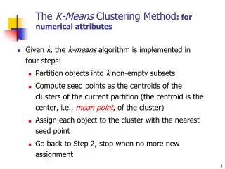
The K-Means Clustering Method : for numerical attributes. Given k , the k-means algorithm is implemented in four steps: Partition objects into k non-empty subsets

E N D
The K-Means Clustering Method: for numerical attributes • Given k, the k-means algorithm is implemented in four steps: • Partition objects into k non-empty subsets • Compute seed points as the centroids of the clusters of the current partition (the centroid is the center, i.e., mean point, of the cluster) • Assign each object to the cluster with the nearest seed point • Go back to Step 2, stop when no more new assignment
10 9 8 7 6 5 4 3 2 1 0 0 1 2 3 4 5 6 7 8 9 10 The K-Means Clustering Method • Example 10 9 8 7 6 5 Update the cluster means Assign each objects to most similar center 4 3 2 1 0 0 1 2 3 4 5 6 7 8 9 10 reassign reassign K=2 Arbitrarily choose K object as initial cluster center Update the cluster means
K-Means • Consider the following 6 two-dimensional data points: • x1: (0, 0), x2:(1, 0), x3(1, 1), x4(2, 1), x5(3, 1), x6(3, 0) • If k=2, and the initial means are (0, 0) and (2, 1), (using Euclidean Distance) • Use K-means to cluster the points.
K-Means • Now we know the initial means: • Mean_one(0, 0) and mean_two(2, 1), • We are going to use Euclidean Distance to calculate the distance between each point and each mean. • For example: • Point x1 (0, 0), point x1 is exactly the initial mean_one, so we can directly put x1 into cluster one.
K-Means • Next we check Point x2 (1, 0) Distance1: x2_and_mean_one = = 1 Distance2: x2_and_mean_two = = Distance1<Distance2, so point x2 is closer to mean_one, Thus x2 belongs to cluster one.
K-Means Similarly for point x3 (1, 1), Distance1: x3_and_mean_one = = Distance2: x3_and_mean_two = = 1 Distance1>Distance2, so point x3 is closer to mean_two, Thus x3 belongs to cluster two.
K-Means Next point x4 (2, 1), • point x4 is exactly the initial mean_two, so we can directly put x4 into cluster two. Next point x5 (3, 1), Distance1: x5_and_mean_one = = Distance2: x5_and_mean_two = = 1 Distance1>Distance2, so point x5 is closer to mean_two, Thus x5 belongs to cluster two.
K-Means Next point x6 (3, 0), Distance1: x6_and_mean_one = = Distance2: x6_and_mean_two = = Distance1>Distance2, so point x6 is closer to mean_two, Thus x6 belongs to cluster two.
K-Means Now the two clusters are as follows: Cluster_One: x1(0, 0), x2(1, 0) Cluster_Two: x3(1, 1), x4(2, 1), x5(3, 1), x6(3, 0) Now update the cluster means: Mean of Cluster_One: mean_one = ((0+1)/2, (0+0)/2) = (0.5, 0) Mean of Cluster_Two: mean_two= ((1+2+3+3)/4, (1+1+1+0)/4) = (2.25, 0.75)
K-Means Now re-assign the points according to the new means: mean_one(0.5, 0) and mean_two (2.25, 0.75) For example, x1 (0,0) Distance1: x1_and_mean_one = = Distance2: x1_and_mean_two = = Distance1 < Distance2, So point x1 should remain in the cluster one. Repeat the same for the other data points.
K-Means After this re-assign iteration: Cluster One: x1(0, 0), x2(1, 0), x3(1, 1) Cluster Two: x4(2, 0), x5(3, 1), x6(3, 0) Now update the cluster means: Mean of Cluster_One: mean_one = ((0+1+1)/3, (0+0+1)/3) = (0.667, 0.33) Mean of Cluster_Two: mean_two = ((2+3+3)/3, (0+1+0)/3) = (2.67, 0.33)
K-Means Now re-assign the points according to the new means: mean_one(0.667, 0.33)and mean_two(2.67, 0.33) … However, after the re-assign process, we find that the clusters remain the same, so we can stop here since there is no change at all. So the final results are : Cluster One: x1(0, 0), x2(1, 0), x3(1, 1) Cluster Two: x4(2, 0), x5(3, 1), x6(3, 0)
Hierarchical Clustering Methods • The partition of data is not done at a single step. • There are two varieties of hierarchical clustering algorithms • Agglomerative – successively fusions of the data into groups • Divisive – separate the data successively into finer groups
Dendrogram • Hierarchic grouping can be represented by two-dimensional diagram known as a dendrogram. 3 Dendrogram 4 5 2 1 3.0 2.0 1.0 4.0 5.0 0 Distance
Distance • Single Linkage • Complete Linkage • Group Average Linkage • Centroid Linkage • Median Linkage
Single Linkage • Also, known as the nearest neighbor technique • Distance between groups is defined as that of the closest pair of data, where only pairs consisting of one record from each group are considered Cluster B Cluster A
(12) 3 4 5 (12) 3 4 5 Dendrogram 2 1 3.0 2.0 1.0 4.0 5.0 0 Distance Find the smallest value, merge them 1 2 3 4 5 1 2 3 4 5 Update Distance
1 and 2 as a whole (12) 3 4 5 (12) 3 4 5 Dendrogram 2 1 3.0 2.0 1.0 4.0 5.0 0 Distance
(12) 3 (4 5) (12) 3 (4 5) 5 4 Repeat: find the smallest one, merge (12) 3 4 5 (12) 3 4 5 Dendrogram 2 1 3.0 2.0 1.0 4.0 5.0 0 Distance
(12) 3 (4 5) (12) 3 (4 5) 5 Dendrogram 4 2 1 3.0 2.0 1.0 4.0 5.0 0 Distance
(12) (3 4 5) (12) (3 4 5) 3 (12) 3 (4 5) (12) 3 (4 5) 5 Dendrogram 4 2 1 3.0 2.0 1.0 4.0 5.0 0 Distance
(12) (3 4 5) (12) (3 4 5) 3 5 Dendrogram 4 2 1 3.0 2.0 1.0 4.0 5.0 0 Distance
(12) (3 4 5) (12) (3 4 5) 3 5 Dendrogram 4 2 1 3.0 2.0 1.0 4.0 5.0 0 Distance
DBSCAN • Traditional Clustering • Can only represent sphere clusters • Cannot handle irregular shaped clusters • DBSCAN • Density-Based Spatial Clustering of Applications with Noise
DBSCAN c d b a e • Given a point p and a non-negative real number , • the -neighborhood of point p, denoted by N(p), is the set of points q (including point p itself) such that the distance between p and q is within .
DBSCAN c d b a e • According to -neighborhood of point p, we classify all points into three types • core points • border points • noise points Given a point p and a non-negative integer MinPts, if the size of N(p) is at least MinPts, then p is said to be a core point. Given a point p, p is said to be a border point if it is not a core point but N(p) contains at least one core point. Given a point p, p is said to be a noise point if it is neither a core point nor a border point.
Example • Consider the following 9 two-dimensional data points: x1(0,0), x2(1,0), x3(1,1), x4(2,2), x5(3,1), x6(3,0), x7(0,1), x8(3,2), x9(6,3) Use the Euclidean Distance with Eps=1 and MinPts = 3 (Eps is short for epsilon: ) Find all core points, border points and noise points, and show the final clusters using DBCSAN algorithm.
Calculate the N(p),-neighborhood of point p • N(x1) = {x1, x2, x7} • N(x2) = {x2, x1, x3} • N(x3) = {x3, x2, x7} • N(x4) = {x4, x8} • N(x5) = {x5, x6, x8} • N(x6) = {x6, x5} • N(x7) = {x7, x1, x3} • N(x8) = {x8, x4, x5} • N(x9) = {x9}
Find all core points according to N(p) • If the size of N(p) is at least MinPts, then p is said to be a core point. • Here the given MinPts is 3, thus the size of N(p) is at least 3. • We can find: • N(x1) = {x1, x2, x7} • N(x2) = {x2, x1, x3} • N(x3) = {x3, x2, x7} • N(x5) = {x5, x6, x8} • N(x7) = {x7, x1, x3} • N(x8) = {x8, x4, x5}
Find all core points according to N(p) • Thus core points are: {x1, x2, x3, x5, x7, x8} • Then according to the definition of border points: given a point p, p is said to be a border point if it is not a core point but N(p) contains at least one core point. N(x4) = {x4, x8} N(x6) = {x6, x5} , here x8 and x5 are core points, So both x4 and x6 are border points. Obviously, x9 is a noise point.
Core points, Border points, Noise points • CorePoints are: {x1, x2, x3, x5, x7, x8} • BorderPoints: {x4, x6} • NoisePoints: {x9}
DBSCAN: The Algorithm • Arbitrary select a point p • Retrieve all points density-reachable from p w.r.t. Eps and MinPts • If p is a core point, a cluster is formed • If p is a border point, no points are density-reachable from p and DBSCAN visits the next point of the database • Continue the process until all of the points have been processed
DBSCAN: Example step by step • Arbitrary select a point p, now we choose x1 • Retrieve all points density-reachable from x1: {x2, x3, x7} • Here x1 is a core point, a cluster is formed. • So we have Cluster_1: {x1, x2, x3, x7} • Next we choose x5, • Retrieve all points density-reachable from x5: {x8, x4, x6}
DBSCAN: Example step by step • Here x5 is a core point, a cluster is formed. • So we have Cluster_2: {x5, x4, x8, x6} • Next we choose x9, x9 is a noise point, noise points do NOT belong to any clusters. • Thus the algorithm stops here.