Download
1 / 33
330 likes | 534 Views
Probabilistic Robotics. Probabilistic Motion Models. Robot Motion. Robot motion is inherently uncertain. How can we model this uncertainty?. Dynamic Bayesian Network for Controls, States, and Sensations. Probabilistic Motion Models.

E N D
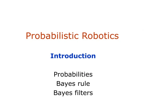
Probabilistic Robotics Probabilistic Motion Models
Robot Motion • Robot motion is inherently uncertain. • How can we model this uncertainty?
Dynamic Bayesian Network for Controls, States, and Sensations
Probabilistic Motion Models • To implement the Bayes Filter, we need the transition model p(x | x’, u). • The term p(x | x’, u) specifies a posterior probability, that action u carries the robot from x’ to x. • In this section we will specify, how p(x | x’, u) can be modeled based on the motion equations.
Coordinate Systems • In general the configuration of a robot can be described by six parameters. • Three-dimensional cartesian coordinates plus three Euler angles pitch, roll, and tilt. • Throughout this section, we consider robots operating on a planar surface. • The state space of such systems is three-dimensional (x,y,).
Typical Motion Models • In practice, one often finds two types of motion models: • Odometry-based • Velocity-based (dead reckoning) • Odometry-based models are used when systems are equipped with wheel encoders. • Velocity-based models have to be applied when no wheel encoders are given. • They calculate the new pose based on the velocities and the time elapsed.
Example Wheel Encoders These modules require +5V and GND to power them, and provide a 0 to 5V output. They provide +5V output when they "see" white, and a 0V output when they "see" black. These disks are manufactured out of high quality laminated color plastic to offer a very crisp black to white transition. This enables a wheel encoder sensor to easily see the transitions. Source: http://www.active-robots.com/
Dead Reckoning • Derived from “deduced reckoning.” • Mathematical procedure for determining the present location of a vehicle. • Achieved by calculating the current pose of the vehicle based on its velocities and the time elapsed.
different wheeldiameters ideal case carpet bump Reasons for Motion Errors and many more …
Odometry Model • Robot moves from to . • Odometry information .
The atan2 Function • Extends the inverse tangent and correctly copes with the signs of x and y.
Noise Model for Odometry • The measured motion is given by the true motion corrupted with noise.
Typical Distributions for Probabilistic Motion Models Normal distribution Triangular distribution
Calculating the Probability (zero-centered) • For a normal distribution • For a triangular distribution • Algorithm prob_normal_distribution(a,b): • return • Algorithm prob_triangular_distribution(a,b): • return
values of interest (x,x’) odometry values (u) Calculating the Posterior Given x, x’, and u • Algorithm motion_model_odometry(x,x’,u) • return p1 · p2 · p3
Application • Repeated application of the sensor model for short movements. • Typical banana-shaped distributions obtained for 2d-projection of 3d posterior. p(x|u,x’) x’ x’ u u
Algorithm sample_normal_distribution(b): • return How to Sample from Normal or Triangular Distributions? • Sampling from a normal distribution • Sampling from a triangular distribution • Algorithm sample_triangular_distribution(b): • return
Normally Distributed Samples 106 samples
103 samples 104 samples 106 samples 105 samples For Triangular Distribution
Algorithm sample_distribution(f,b): • repeat • until ( ) • return Rejection Sampling • Sampling from arbitrary distributions
Example • Sampling from
sample_normal_distribution Sample Odometry Motion Model • Algorithm sample_motion_model(u, x): • Return
Start Sampling from Our Motion Model
Equation for the Velocity Model Center of circle: with
Approximation: Map-Consistent Motion Model
Summary • We discussed motion models for odometry-based and velocity-based systems • We discussed ways to calculate the posterior probability p(x| x’, u). • We also described how to sample from p(x| x’, u). • Typically the calculations are done in fixed time intervals t. • In practice, the parameters of the models have to be learned. • We also discussed an extended motion model that takes the map into account.