Download

1 / 24
240 likes | 412 Views
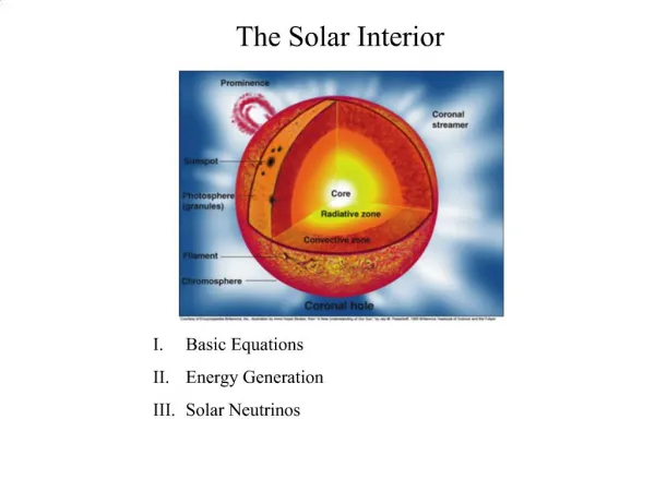
Understanding the Connection Between Magnetic Fields in the Solar Interior and the Solar Corona. George H. Fisher Space Sciences Laboratory UC Berkeley. Overview. The Focus:. Active region magnetic fields in the convective envelope below the photosphere

E N D
Understanding the Connection Between Magnetic Fields in the Solar Interior and the Solar Corona George H. Fisher Space Sciences Laboratory UC Berkeley
The Focus: • Active region magnetic fields in the convective envelope below the photosphere • Quiet Sun magnetic fields, the turbulent dynamo, and X-ray emission in main sequence stars • Connecting observations of magnetic field in the solar photosphere to numerical models of the solar corona
The Emergence and Decay of Active Region Magnetic Fields Below the Photosphere The dangers of over-interpreting 2D results: How much field line twist does a flux tube need to prevent its fragmentation?
The Emergence and Decay of Active Region Magnetic Fields in the Convection Zone The effects of convective turbulence on active region-scale magnetic fields below the surface: What field strength is necessary for a flux rope to retain its cohesion?
The Transport of Magnetic Flux The effects of convective turbulence on initially “neutrally-buoyant” active region-scale magnetic structures with field strengths near the cohesion limit: How rapidly is magnetic flux transported to the base of the convection zone?
The Turbulent Dynamo • This type of model should not be confused with a global dynamo model --- in our case, there is no need for an interface layer, rotation (differential or otherwise), or prescribed flows. • Our work differs from that of Cattaneo (1999) in that our domain is highly stratified --- but like his Boussinesq calculation, we find that our small seed field grows exponentially until it saturates at ~7% of the total kinetic energy of the computational domain. Compute time: 5.5 CPU months (2.4 GHz Xeon)
The Turbulent Dynamo and X-ray Flux in Stars • We use simple stellar structure theory (MLT) to scale our simulations to the outer layers of main sequence stars (in the F0 to M0 spectral range) --- this allows us to estimate the unsigned flux on the surface of “non-rotating” reference stars. • With these estimates, we use the empirical relationship of Pevtsov et al. (2003) to estimate the amount of X-ray emission resulting from such a turbulent dynamo.
The Turbulent Dynamo and X-ray Flux in Stars • Our results compare well with the observed lower limits of X-ray flux (and when scaled to chromospheric levels, compare well with the observed lower limits of Mg II flux • Thus, we suggest that dynamo action of a non-rotating convective envelope can provide a viable alternative to acoustic heating as a mechanism for the observed “basal” emission level seen in the chromopsheric and coronal emission of main sequence stars
To what extent can we determine the flows in an active region by observing changes in the magnetic field at the photosphere?
The LCT, FLCT techniques • LCT schema in use today have one central idea: proper motions of features in 2 successive images - whether G-band filtergrams, H images, or photospheric magnetograms - separated in time by t are found by maximizing a cross-correlation function, or minimizing an error function between sub-regions of the images. The concept is generally attributed to November & Simon (1988). • The FLCT method (which we developed) is similar. For each pixel, we: • multiply each of the 2 images to be correlated by a Gaussian, of width , centered at that pixel; crop the resulting altered images 1 and 2 by chopping the insignficant parts of the images; • compute the cross-correlation function between the two cropped images using standard Fast Fourier Transform (FFT) techniques; • use cubic-convolution interpolation to find the shifts in x and y that maximize the cross-correlation function to one of two precisions (chosen by the user), either 0.1 or 0.02 pixel; and • use the shifts in x and y and t between images to find the intensity features' apparent motion along the solar surface.
The Demoulin & Berger Interpretation of LCT • Degeneracy: Motions parallel to B do not directly affect apparent motion of magnetic features. • Apparent horizontal motion ULCT is from a combination of horizontal motions and vertical motions acting on non-vertical fields. Flows parallel to B don’t affect the motion of Magnetic Features. Therefore we consider only flows normal to B, and set v•B=0. This constraint, plus the Demoulin & Berger interpretation, leads to this solution for v and vz:
The Ideal MHD Induction Equation • How can we ensure that LCT-determined velocities are physically consistent with the magnetic induction equation? • Only the z-component of the induction equation contains no unobservable vertical derivatives: Now, substitute in the Demoulin & Berger hypothesis The ideal MHD induction equation simplifies to this form:
ILCT – Use LCT to constrain solutions of the induction equation • Take 2D divergence, then z-component of the curl of this definition, and make the approximation that U=ULCT: Let Applying the above definition for BzU then guarantees that the resulting solution for U will obey the induction equation.
Apply ILCT to IVM vector magnetogram data for AR 8210 • Vector magnetic field data enables us to find 3-D flow field from ILCT via the equations shown on slide 5. Transverse flows are shown as arrows, up/down flows shown as blue/red contours.
Must have some kind of initial conditions: • Use Force-free field to initialize field in computational volume
Time dependent boundary conditions for the coronal MHD code • Write a separate dynamical code for determining boundary evolution (about 4 zones deep) • Solve magnetic induction, and continuity equations • Substitute ILCT-derived flow field for the momentum equation (this provides the data driving) • Fully couple the coronal MHD code to the boundary code
Illustration of 2 coupled codes • Transparent planes at the bottom illustrate the boundary evolution code
Toward a Data-driven Simulation of AR-82104 hrs of solar time, corresponding to the vector magnetogram time sequence
Data Driven Simulations:Plans for future • Find longer vector magnetogram sequences so can run simulation longer • Greatly expand the simulation box size; extend to spherical chunks • Include a shearing of vx, vy in z direction in boundary code to account for observed changes in Bx and By. • Experiment with using LOS magnetograms