Download
1 / 30
300 likes | 322 Views
Discover how the Earth's vibrations are represented through normal modes, from standing waves to surface wave packets, and learn about the complex arithmetic involved in seismology.

E N D
Seismology Part VIII: Normal Modes and Free Oscillations
So far we have been dealing with unbounded media, and all the waves are traveling waves (they simply propagate from one point to another). However, the Earth is a finite medium, and so it should happen that certain frequencies will constructively interfere. These are call the normal modes of vibration of the Earth. Because they are excited by sources internal to the medium, they are also called free oscillations. We can see what happens in the simple 1D case of a string of length L tied at the ends (similar results occur for any musical instrument). The general solution to the 1D wave equation is:
We set the boundary conditions: u(0,t) = u(L,t) = 0. At x=0: and so C1 = -C2 and C3 = -C4. Then at x=L: Nontrivial solutions are found with the argument to the sine is a multiple of .
These are the eigenfrequencies of the system, and the solutions for u(x,t) with these frequencies are the eigenfunctions of the system.
Note that although this solution seems to be particular to a certain kind of wave (standing wave), in fact we can generate the solution to any arbitrary disturbance (including traveling waves) by summing over properly weighted normal modes: Thus, surface waves that traverse the Earth several times can be thought of as packets of waves moving about the Earth or as eigenfunctions of the Earth’s vibrations. By definition, the normal modes represent ALL of the possible vibrations in the planet (or any body) and so it should in theory be possible to construct any wave by superimposing them.
The best way to think about what happens on a sphere is to view the waves as solutions to the wave equation on terms of spherical harmonics. Let’s consider how this would work for a fluid earth (so only compressional waves). The solid earth case is analogous but there’s a lot more arithmetic involved. First, we have to write the wave equation in a spherical coordinate system (r, instead of (x, y, z): In this case S is the pressure in the fluid (so should be zero at the surface). Note also that our sphere is also non-rotating. (why is that important?)
Solve the above using separation of variables (the usual trick): S(r, tR(r)T(t) We’ll let T(t) = e-it.
Thus, eliminating T: or The left hand side is independent of , so the right hand side must be a constant. If we choose this to be m2 then
which has the general solution = eim = cos(m) + isin(m) Note that m must be an integer (0, +-1, +-2, etc.) to preserve the 2 spatial periodicity on a sphere. We now have
Each side must be equal to the same constant. Let's call that K, so that Let's see what happens to the equation when m=0. or
Then Hence we have his is called the Legendre equation. Here's how to solve it: we presume that we can find a polynomial representation of (x) such that:
So Identifying equal powers of x in the above gives:
or in general for the xk term: From the first equality, we see that k=0 or k=1. The k=1 solutions are a subset of k=0, so we choose k=0 for the most general case. Thus Note that
so the series will converge as long as -1<x<1 or 0< (i.e. almost everywhere on earth). What about x = 1 or x = -1? It turns out that the polynomial for will diverge unless by some chance an even suffix bi and an odd suffix bi is zero, which of course means that the sum is no longer infinite (so convergence is guaranteed - duh). Looking above at the definition of b, we see that any bi+2 will be equal to zero for a nonzero bi only if K = (i)(i+1). Thus, it must be that K is the product of two successive integers! Let K = l(l+1). Then If l is even then it is a sequence of even suffixed b that make up the solution and we must require that b1 = 0 (so all odd guys are zero). Similarly , if l is odd then the sequence is odd-suffix bi and b0 = 0. In either case, is a polynomial of order l.
Typically, we choose bo or b1 by requiring (x) = 1 for x = 1 (i.e., = 0 degrees). The resulting polynomials are called Legendre polynomials, and they have the general form: stopping with either x or 1(times a constant) as the last term. The first few polynomials are:
They can also be calculated using Rodrigues' formula: Ok, so how about when m is not 0? In this case, our substitution trick gives: It turns out that the polynomial approach above bogs down, and the way to solve this guy is to look at what happens when x gets close to +-1. We also factor such that:
and determine that A(x) satisfies the ODE: This equation can be expanded just like we did before: and we get a similar recursive relationship for c: Note that when m=0 we revert to our equation for bi. As before: ci+2 = 0 for some i, and additionally if c has an even index, then we require that c1 = 0, and if c has an odd index, then c0 = 0. Thus, K has the eigenvalues:
or again that K is the product of consecutive integers. If we let l = i + m as before, then because i > 0 it must be that m < l. Thus, there is an constraining relation between the order of the solution for Q and the latitudinal order m. However, note that K can have the same eigenvalues for different choices of m, so there is some independence. If we differentiate the original Legendre polynomial equation m times we get:
which looks just like the equation for A(x), where we identify A(x) as the mth derivative of Pl. Thus: These mth derivatives of the Legendre polynomials are called associated Legendre functions. From the Rodrigues formula above, we see that which is valid for all l and all m such that -l<m<l.
We often combine the solutions for and (along with a normalization factor) to produce the function: Now, let's get an expression for R(r). Substituting our value of K in the above gives: is a form of the Bessel equation, which has solutions called spherical Bessel functions or Hankel functions of the form:
where in this case x = r/c. Note that for l = 0 Note that for l = 2
Because this is a pressure wave (the wave equation is posed with pressure as the variable), the free surface condition is that R(ro) = 0. Thus for l = 0 it must be that: from which the eigenfrequencies nl for this case are: where n = 0 is the fundamental mode and n > 0 are the overtones. Note that for any choice of l (and mode n), because -l < m < l, there are 2l-1 possible choices of m that go with the same eigenfrequency. Thus, a single frequency will correspond to several different free oscillations. This is referred to as frequency degeneracy.
Note that l = 0 is a purely radial mode, because the associated and motions are zero. In a sphere, we have to concern ourselves with two basic kinds of vibration: Spheroidal: involving motion in the radial direction Toroidal: motion parallel to the surface. There is a useful nomenclature developed to classify the different spherical modes: nSl nTl The index on the left indicates the number of zero crossings.
The index on the right indicates the angular order or degree of the harmonic. A node at the surface will appear every /n degrees, or equivalently motion of the same type will appear every 2/n degrees. • Some examples: • 0S0 The whole Earth expanding and contracting. At every point the radius is increasing and decreasing in phase. • 1S0 Imagine the same picture as 0S0, but the inner part of the Earth is contracting while the outer half is expanding. • 0S1 Would be one half of the Earth contracting while the other half is expanding. This would result in a net change in the center of mass of the Earth, and hence cannot be excited by an internal source. • 0S2 is sometimes called the “football” mode. Imagine the Earth compressing at the poles and expanding at the equator
0T0 Undefined – can’t work because toroidal modes by definition have to repeat every 2 • 0T1 Nonphysical – would cause the earth’s rotation to increase and decrease, which would violate conservation of angular momentum • 0T2 One hemisphere twists in one direction; other hemisphere in opposite direction. • Depth sensitivity: • Generally complicated, but fundamental modes have energy concentrated in the upper mantle. • Splitting: • Caused mostly by rotation (Coriollis and angular momentum). Multiplets split into singlets.