Download
1 / 25
250 likes | 274 Views
Explore arbitrary experimental designs with specific stimuli, response events, and convolution techniques for predicting responses. Investigate the shift-invariance and additivity principles in signal processing. Learn about Fourier Transforms and convolution theorems in functional MRI analysis.

E N D
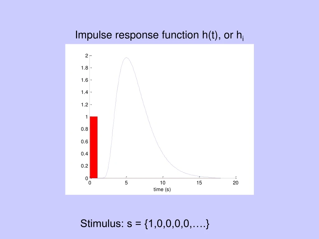
Impulse response function h(t), or hi Stimulus: s = {1,0,0,0,0,….}
Two events 2.5 2 1.5 1 0.5 0 0 5 10 15 20 time (s) Stimulus: s = {1,0,0,0,1,0….}
Two events Stimulus: s = {1,0,0,0,.5,0….}
7 6 5 4 3 2 1 0 0 50 100 150 200 250 time (s) Arbitrary experimental design Stimulus: s = {0,0,1,0,1,1,0,0,1,……}
3.5 3 2.5 2 1.5 1 0.5 0 0 5 10 15 20 25 30 35 40 time (s) Response at time i=18 s4h14 + s6h12 + s10h8 Response at time i s1hi-1 + s2hi-2 + …+ si-1h1 Stimulus: s = {0,0,0,1,0,1,0,0,0,1,0,0,…}
2 2 1.5 1.5 1 1 0.5 0.5 0 0 0 20 40 60 80 0 20 40 60 80 time (s) time (s) 0.2 0.2 0.15 0.15 0.1 0.1 0.05 0.05 0 0 0 20 40 60 80 0 20 40 60 80 time (s) time (s) 6 4 2 0 0 10 20 30 40 50 60 70 80 time (s)
Response R Design Matrix X Impulse response h x =
if then
Time-contrast separability Boynton, G.M., et al., J Neurosci, 1996. 16(13): p. 4207-21.
Shift-invariance response to 6 sec pulse shift and duplicate 3 3 0 0 -3 -3 0 10 20 30 40 0 10 20 30 40 response to 12 sec pulse predict 12 sec from 6 sec pulses 3 3 0 0 -3 -3 0 10 20 30 40 0 10 20 30 40 Time (sec) Intensity Boynton, G.M., et al., J Neurosci, 1996. 16(13): p. 4207-21.
3 predicts 6 gmb 3 Response to pulsed stimulus Prediction from shift and sum 0 -3 0 10 20 30 40 3 predicts 12 6 predicts 12 3 3 0 0 -3 -3 0 10 20 30 40 0 10 20 30 40 3 predicts 24 6 predicts 24 12 predicts 24 3 3 3 0 0 0 -3 -3 -3 0 10 20 30 40 0 10 20 30 40 0 10 20 30 40 time (sec) Shift-invariance Intensity Boynton, G.M., et al., J Neurosci, 1996. 16(13): p. 4207-21.
Additivity single stimulus paired same time SOA Stimuli: 0.5 c/deg, 8 Hz counterphase 30 deg 1sec duration 48 repetitions per condition 30 deg
Nonlinearity after subtracting response to first pulse: single stimulus paired same
single stimulus paired same paired orthogonal after subtracting response to first pulse:
What does convolution have to do with sinusoids and Fourier Transforms? Convolution of sinusoid is a sinusoid:
Convolution changes the amplitude and phase of a sinusoid – but NOT the frequency
Fourier transform: Convolution of sinusoid is a sinusoid: Combined: Convolution of a function can be expressed via amplitude scaling and phase shifts of the function’s Fourier components.
The amplitude scaling and phase shifts of the function’s Fourier components are determined by the Fourier transformation of the impulse response function. FFT of h(t)
The convolution theorem: FFT of s(t) S(w) stimulus: s(t) FFT of h(t) H(w) HDR: h(t) convolution multiplication IFFT response: f(t)*h(t) S(w) H(w)
fft of stimulus stimulus 3 0.12 2.5 0.1 0.08 2 amplitude 1.5 0.06 1 0.04 0.5 0.02 0 0 0 40 80 120 6 12 18 24 30 36 Time (sec) Cycles/scan response fft of response 0.1 1.2 1 0.08 0.8 0.06 amplitude 0.6 0.04 0.4 0.02 0.2 0 0 0 40 80 120 6 12 18 24 30 36 Time (sec) Cycles/scan
Example: simple block design 10 9 8 7 6 5 4 3 2 1 0 0 50 100 150 200 250 time (s) Stimulus: s = {1,1,1,…,0,0,0,…,1,1,1,…,0,0,0,…}
3 0.8 2.5 0.6 2 amplitude 1.5 0.4 1 0.2 0.5 0 0 0 40 80 120 160 200 240 6 12 18 24 30 36 Time (sec) Cycles/scan 0.8 1.2 1 0.6 0.8 amplitude 0.4 0.6 0.4 0.2 0.2 0 0 0 40 80 120 160 200 240 6 12 18 24 30 36 Time (sec) Cycles/scan fft of stimulus stimulus response fft of response
fMRI amplitude for different stimulus frequencies and contrasts
fMRI amplitude at different frequencies for a 30 second period stimulus