Diving Deeper into Chaining and Linear Probing
270 likes | 285 Views
Explore k-universal hashing, separate chaining, linear probing, and more concepts in hashing. Learn about load factors, linear probing milestones, expected costs, and provable facts. Dive deeper into the world of hashing!

Diving Deeper into Chaining and Linear Probing
E N D
Presentation Transcript
Diving Deeper into Chaining and Linear Probing COMP 480/580 17th Jan 2019
Announcements • Assignment 1 will be released today and is, due 2 weeks from now, 31st Jan. Submission via Canvas. • Tomorrow is the deadline to pick project over final exams. No email from you means you are choosing final exam by default. • All deadlines are 11:59pm CT on the given day.
Refresher • k-universal hashing family • A hash function is k-universal if for any set • For h chosen uniformly from are independent random variables. • OR • We saw 2-universal family. Generally for k-independent family we need polynomial in k • h(x) = ) mod P mod R • Higher independence is harder to achieve from both computation and memory perspective.
Separate Chaining. 41 • key space = integers • TableSize = 10 • h(K) = K mod 10 • Insert: 7, 41,18, 17 17 7 18
What we saw? • m objects inserted into array of size n • Expected length of chain • The quantity is termed as load factor denoted by • Expected addition and search time • Worst Case: m • Is this satisfactory? Are there better variants of chaining? How much better?
What is a good running time? • Log(n). • Natural question: What is the probability that there exist a chain of size . More information than expected value!!
Counting and Approximations! Theorem: For the special case with m=n, with probability at least 1-1/n, the longest list is O(ln n / ln lnn). Proof: • Let Xi,k= Indicator of {key ihash to slot k}, Pr(Xi,k=1) = 1/n • The probability that a particular slot k receives >κ keys is (letting m=n) (assuming lot if independence) • If we choose κ= 3 ln n / ln lnn, then κ! > n2 and 1/κ! < 1/n2. • Thus, the probability that any n slots receives >κ keys is < 1/n.
Better? • Can we do better? • Use two hash functions, insert at the location with smaller chain. • Assignment: Using m=n slots, with probability at least 1-1/n, the longest list is O(log logn). Exponentially better!!
Linear Probing F(i) = i • Probe sequence: 0th probe = h(k) mod TableSize 1th probe = (h(k) + 1) mod TableSize 2th probe = (h(k) + 2) mod TableSize . . . ith probe = (h(k) + i) mod TableSize
Probing or Open Addressing Insert: 38 19 8 109 10 • Linear Probing: after checking spot h(k), try spot h(k)+1, if that is full, try h(k)+2, then h(k)+3, etc.
Major Milestones of Linear Probing • In 1954, Gene Amdahl, Elaine McGraw, and Arthur Samuel invent linear probing as a subroutine for an assembler. • In 1962, Don Knuth, in his first ever analysis of an algorithm, proves that linear probing takes expected time O(1) for lookups if the hash function is truly random (n-wise independence). • In 2006, Anna Pagh et al. proved that 5-independent hash functions give expected constant-time lookups. • In 2007, Mitzenmacher and Vadhan proved that 2-independence will give expected O(1)-time lookups, assuming there’s some measure of randomness in the keys.
Linear Probing in Practice • In practice, linear probing is one of the fastest general-purpose hashing strategies available. • This is surprising – it was originally invented in 1954! It's pretty amazing that it still holds up so well. • Why is this? • Low memory overhead: just need an array and a hash function. • Excellent locality: when collisions occur, we only search in adjacent locations. • Great cache performance: a combination of the above two factors
Analyze Expected cost of Linear Probing • For simplicity, let’s assume a load factor of α = = ¹/₃. • What happens to linear probing of • Contrast with chaining. • A region of size m is a consecutive set of m locations in the hash table. • An element q hashes to region R if h(q) ∈ R, though q may not be placed in R. • On expectation, a region of size should have at most ¹/₃ elements hash to it. • It would be very unlucky if a region had twice as many elements in it as expected. A region of size is overloaded if at least ²/₃ elements hash to it.
A Provable Fact • Theorem: The probability that the query element q ends up between and steps from its home location is upper-bounded by • c · Pr[ the region of size centered on h(q) is overloaded ] for some fixed constant c independent of s. • Proof: Set up some cleverly-chosen ranges over the hash table and use the pigeonhole principle. See Thorup’s lecture notes. • https://arxiv.org/abs/1509.04549
Overall we can write the expectation as • E(lookup time) = If we can bound Pr[ the region of size centered on h(q) is overloaded ]
Recall • A region is a contiguous span of table slots, and we’ve chosen α = ¹/₃. • An overloaded region has at least ⅔ · 2ˢ elements in it. • Let the random variable Bₛ represent the number of keys that hash into the block of size 2ˢ centered on h(q) (q is our search query). • We want to know Pr[ Bₛ ≥ ⅔ · ]. • Assuming our hash functions are at least 2-independent (why?), we have • E[Bₛ] = ⅓ · 2ˢ. • Pr[ Bₛ ≥ ⅔ · ] is equivalent to Pr[ Bₛ ≥ 2·E[Bₛ] ]. • Thus, looking up an element takes, on expectation, at least
Apply Markov’s • No Assumptions!! • Pr[ Bₛ ≥ 2·E[Bₛ] ] • . BAAAAAAD • (we want to decay faster than to get anything interesting)
Concentration Inequalities (Last Class) • Markov’s Inequality • Pr • Chebyshev’s • Pr • Chernoff Bounds. • Pr A fair coin is tossed 200 times. How likely is it to observe at least 150 heads? ❖ Markov: ≤ 0.6666 ❖ Chebyshev: ≤ 0.02 ❖ Chernoff: ≤ 0.017
Concentration Inequalities (Last Class) • Markov’s Inequality • Pr • Chebyshev’s • Pr ( ) • Chernoff Bounds. ( is sum of i.i.d variables) • Pr More Independence More Resources in Hash Functions
Can we bounds the variance? • Define indicator variable: if elements maps to block of size 2ˢ centered at h(q) =
Variance • Var[] = • E[] = • = • = (assuming 3-independence!!) • What does 3-independence buys us < (why? … do the math) So Var[] []
Pr The bound is tight for 3-independence
Going Beyond: 4th Moment Bound • Pr • Assignment: Prove that expected cost of linear probing is O(1) assuming 5-independence using the above 4th moment bounds.
In practice 2-independence suffice? • In 2007, Mitzenmacher and Vadhan proved that 2-independence will give expected O(1)-time lookups, assuming there’s some measure of randomness in the keys. • Assignment for Grads: Read this paper.
Cuckoo Hashing • Worst case of both chaining and probing is O(n). Expected is O(1). • Includes both insertion and searching. • Can we sacrifice insertions for worst case O(1) searching? • YES • Cuckoo Hashing
In practice • In practice Cuckoo hashing is about 20-30% slower than linear probing which is the fastest of the common approaches.
