Download
1 / 32
320 likes | 369 Views
Explore a geometric approach for monitoring large-scale distributed data systems by utilizing drift vectors, convex hulls, and local constraints. Balancing accuracy and performance, shape sensitivity, prediction-based monitoring, safe zones, and improving monitoring methods. Discover how geometric methods save communication and resources while maintaining precision and latency.

E N D
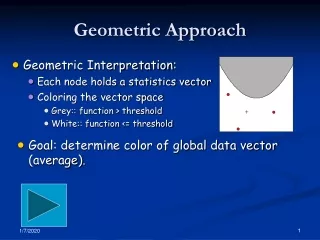
Geometric Approach • Geometric Interpretation: • Each node holds a statistics vector • Coloring the vector space • Grey:: function > threshold • White:: function <= threshold • Goal: determine color of global data vector (average).
Bounding the Convex Hull • Observation: average is in the convex hull • If convex hull monochromatic then average too • But – convex hull may become large
Drift Vectors • Periodically calculate an estimate vector - the current global • Each node maintains a drift vector – the change in the local statistics vector since the last time the estimate vector was calculated • Global average statistics vector is also the average of the drift vectors
The Bounding Theorem [SIGMOD’06] • A reference point is known to all nodes • Each vertex constructs a sphere • Theorem: convex hull is bounded by the union of spheres • Local constraints!
Basic Algorithm • An initial estimate vector is calculated • Nodes check color of drift spheres • Drift vector is the diameter of the drift sphere • If any sphere non monochromatic: node triggers re-calculation of estimate vector
Reuters Corpus (RCV1-v2) • 800,000+ news stories • Aug 20 1996 -- Aug 19 1997 • Corporate/Industrial tagging n=10 10 nodes, random data distribution
Trade-off: Accuracy vs. Performance • Inefficiency: value of function on average is close to the threshold • Performance can be enhanced at the cost of less accurate result: • Set error margin around the threshold value
Balancing • Globally calculating average is costly • Often possible to average only some of the data vectors.
Shape Sensitivity [PODS’08] • Fitting cover to Data • Fitting cover to threshold surface • Specific function classes
Fitting Cover to Threshold Surface --Reference Vector Selection
Distance Fields Skeleton, Medial Axis
ΔVp2 ΔV2 ΔVp1 ΔV1 ΔV3 ΔVp3 ΔVp5 ΔVp4 ep e ΔV5 ΔV4 Prediction-Based Geometric Monitoring [SIGMOD’12] f(v(t)) > T v(t) • Stricter local constraints if local predictions remain accurate • Keeping up with v(t) movement
Local Constraints Safe Zones! Let the nodes communicate only when “something happens” Tell me only if your measurement is larger than 50! Send me your current measurements!
Local Distributions Reasonable to assume future data will behave similarly… These Safe Zones save more communication!
Example: Air quality monitoring What are the optimal Safe Zones…?
The Optimization Problem Is this Convex? Is this Linear? How many constraints are these? BAD NEWS: This problem is NP-hard.
The Optimization Problem X • Step 3: Use non-convex optimization toolboxes (e.g. Matlab’s “fmincon”). • These toolboxes use sophisticated Gradient Descent algorithms and return close-to-optimal results.
Data Set How the data looks like
Ratio Queries Example of triangular Safe Zones
Improvement over convex-hull cover method 5’000 hours Up to 200 nodes were involved in the experiment. The average improvement was by a factor of 17.5 Why do we improve so much?
Chi-Square Monitoring (5D) Examples of axis aligned boxes as Safe Zones
Improvement over GM 1’000 hours 90 nodes The improvement over the Geometric Method gets more substantial in higher dimensions.
Biclique: Non-Convex Safe Zones Safe Zone Algorithm (for 2 nodes): Take the data points, build a bipartite graph(how?), find the maximal Biclique, these are your Safe Zones!
Conclusions • Local filtering for large-scale distributed data systems • Saving in communication is unlimited • Bounded only by the aggregate over system lifetime • Saving bandwidth, central resources, power. • Not necessary to sacrifice precision and latency • Less communication more Privacy