Download
1 / 55
560 likes | 639 Views
Explore wind-driven circulation, oceanic gyres, Gulf Stream currents, vorticity dynamics, Stommel and Munk models, and surface current measurements via surface drifters. Learn about the Sverdrup Relation and its application in oceanography. Discover insights into surface winds, subtropical gyres, Rossby waves, and mesoscale eddies through observational data. Dive deep into the complexities of current measurements and the interplay between wind patterns and ocean currents.

E N D
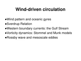
Wind-driven circulation ●Wind pattern and oceanic gyres ●Sverdrup Relation ●Western boundary currents: the Gulf Stream ●Vorticity dynamics: Stommel and Munk models ●Rossby wave and mesoscale eddies
Surface current measurement from ship drift Current measurements are harder to make than T&S The data are much sparse.
More recent equipment: surface drifter a platform designed to move with the ocean current
Annual Mean Surface CurrentNorth Atlantic, 1995-2003 Drifting Buoy Data Assembly Center, Miami, Florida Atlantic Oceanographic and Meteorological Laboratory, NOAA
Annual Mean Surface current from surface drifter measurements Indian Ocean, 1995-2003 Drifting Buoy Data Assembly Center Miami, Florida Atlantic Oceanographic and Meteorological Laboratory NOAA
Annual Mean Surface CurrentPacific Ocean, 1995-2003 Drifting Buoy Data Assembly Center, Miami, Florida Atlantic Oceanographic and Meteorological Laboratory, NOAA
Schematic picture of the major surface currents of the world oceans Note the anticyclonic circulation in the subtropics (the subtropical gyres)
Surface winds and oceanic gyres: A more realistic view Note that the North Equatorial Counter Current (NECC) is against the direction of prevailing wind.
Mean surface current tropical Atlantic Ocean Note the North Equatorial Counter Current (NECC)
Consider the following balance in ocean of depth h , Sverdrup Relation Consider the following balance in an ocean of depth h of flat bottom , Integrating vertically from –h to 0, we have (neglecting bottom stress and surface height change) (1) (2) where and Differentiating , we have and Using continuity equation , Sverdrup relation we have and ,
and More generally, Since , we have set x =0 at the eastern boundary,
Mass Transport Since Let , , where ψ is stream function. Problem: only one boundary condition can be satisfied.
Alternative derivation of Sverdrup Relation Construct vorticity equation from geostrophic balance (1) (2) Integrating over the whole ocean depth, we have is the entrainment rate from the Ekman layer where at 45oN The Sverdrup transport is the total of geostrophic and Ekman transport. The indirectly driven Vg may be much larger than VE.
In the ocean’s interior, for large-scale movement, we have the differential form of the Sverdrup relation i.e., ζ<<f
A more general form of the Sverdrup relation Lower Ekman layer Spatially chaning sea surface height η and bottom topography zB and pressure pB. Assume atmospheric pressure pη≈0. Let , Integrating over the vertical column, we have Taking into account of these factors, the meridional transport can be derived as , where ,
Vorticity Equation In physical oceanography, we deal mostly with the vertical component of vorticity , which is notated as From horizontal momentum equation, (1) (2) Taking , we have
Considering the case of constant ρ. For a shallow layer of water (depth H<<L), u and v are not function of z because the horizontal pressure gradient is not a function of z. (In general, the vortex tilting term, is usually small. Then we have the simplified vorticity equation Since the vorticity equation can be written as (ignoring friction) ζ+f is the absolute vortivity
Assume geostrophic balance on β-plane approximation, i.e., (β is a constant) Vertically integrating the vorticity equation we have The entrainment from bottom boundary layer The entrainment from surface boundary layer We have where
Quasi-geostrophic vorticity equation For , we have and and where (Ekman transport is negligible) Moreover, We have where
Non-dmensional equation Non-dimensionalize all the dependent and independent variables in the quasi-geostrophic equation as where For example, The non-dmensional equation where , nonlinearity. , , , bottom friction. , lateral friction. ,
Interior (Sverdrup) solution If ε<<1, εS<<1, and εM<<1, we have the interior (Sverdrup) equation: (satistfying eastern boundary condition) (satistfying western boundary condition) Example: Let , . Over a rectangular basin (x=0,1; y=0,1)
Westward Intensification It is apparent that the Sverdrup balance can not satisfy the mass conservation and vorticity balance for a closed basin. Therefore, it is expected that there exists a “boundary layer” where other terms in the quasi-geostrophic vorticity is important. This layer is located near the western boundary of the basin. Within the western boundary layer (WBL), , for mass balance The non-dimensionalized distance is , the length of the layer δ <<L In dimensional terms, The Sverdrup relation is broken down.
The Stommel model Bottom Ekman friction becomes important in WBL. , εS<<1. at x=0, 1; y=0, 1. (Since the horizontal friction is neglected, the no-slip condition can not be enforced. No-normal flow condition is used). Interior solution In the boundary layer, let ( ), we have
The solution for is , . A=-B , ξ→∞, ( can be the interior solution under different winds) , For , , . For , , .
The dynamical balance in the Stommel model In the interior, Vorticity input by wind stress curl is balanced by a change in the planetary vorticity f of a fluid column.(In the northern hemisphere, clockwise wind stress curl induces equatorward flow). In WBL, , Since v>0 and is maximum at the western boundary, the bottom friction damps out the clockwise vorticity. Question: Does this mechanism work in a eastern boundary layer?
Munk model Lateral friction becomes important in WBL. Within the boundary layer, let , we have , Wind stress curl is the same as in the interior, becomes negligible in the boundary layer. For the lowest order, . If we let , we have . And for , . . The general solution is Since , C1=C2=0.
Total solution Using the no-slip boundary condition at x=0, (K is a constant). .to , Considering mass conservation K=0 Western boundary current
Vertical structure of the ocean: Large meridional density gradient in the upper ocean, implying significant vertical shear of the currents with strong upper ocean circulation