Download
1 / 27
270 likes | 432 Views
GFDL’s Coupled and Earth System Model Developments. High-resolution Atmosphere and Oceans horizontal (capturing regional, other fine-scale details), vertical (capturing the stratosphere)

E N D
GFDL’s Coupled and Earth System Model Developments • High-resolution Atmosphere and Oceans horizontal (capturing regional, other fine-scale details), vertical (capturing the stratosphere) • Climate Models graduating onto Earth Systems Model, including interactive Atmospheric Chemistry (capturing Climate – Air Quality nexus) and Biogeochemistry (capturing Carbon-Climate feedbacks) • Need for comprehensiveness and realism in representation of processes
Model development strategy within GFDL: 2 pipelines developed in tandem push atmospheric and oceanic climate models to higher resolution, while developing and utilizing lower resolution Earth System Models Precip in 25 km model Surface NOX in AM3 (200 km) Earth system/ comprehensiveness pipeline Resolution pipeline Merge in future
Winter mean precipitation in Western U.S. in 50km model 200 km res. 50 km res. Observations 2 deg. 1/2 deg. Annual mean precipitation in Europe 200km 50km
GFDL Model rainfall Current generation High-Resolution To resolve societally and physically relevant scales: High-res. atmosphere, ocean, coupled models being developed at GFDL Observed SST and Wind Developing generation Model data: S.J. Lin, I. Held, M. Zhao From Vecchi, Xie and Fischer (2004, J. Clim)
High resolution simulation of Southern Ocean (Hallberg and Gnanadesikan, JPO, 2006) Small vortices affect oceanic carbon uptake heat, transport of heat towards Antarctic continent, marine ecology of Southern Ocean
Development Pathway:Coupled Model for AR5 2008 CM3 = AM3 + LM3 + CM2.1 ICE/OCEAN 5yr/day on 500PEs 2400 CPUhr/yr ESM2.1 = CM2.1 + LM3V + OBGC CM2M = CM2.1 with MOM+ ESM2M CM2G = CM2.1 with GOLD ESM2G 8yr/day on 140PEs 425 CPUhr/yr 10yr/day on 120PEs 300 CPUhr/yr
Why two ocean models? • z-coordinate better in weakly stratified regions • -coordinate better on sloping bottom Role of ocean in transient climate change?
LM2 -> LM3 Land Model • Dynamic vegetation • Subgrid land-use heterogeneity • Distinct treatment of ground, vegetation, & canopy air • Soil water dynamics (liquid & frozen) • Multilayer snow pack • River network with capacity for tracers and temperature
Decadal Predictability Research • Ongoing studies with CM2 model to develop improved understanding of • mechanisms of decadal variability • decadal scale predictability arising from internal variability • Development and use of higher resolution coupled models. Want this to be focus of variability and predictability research • New coupled assimilation system
North Atlantic Temperature Atlantic Meridional Overturning Circulation (AMOC) What will the next decade or two bring? Warm North Atlantic linked to … Drought More rain over Sahel and western India More intense hurricanes • Two important aspects: • Decadal-multidecadal fluctuations • Long-term trend
Simulated North Atlantic AMOC Index Aerosol only forcing All forcings Greenhouse gas only forcing
Projected Atlantic SST Change (relative to 1991-2004 mean) Can we predict which trajectory the real climate system will follow? Results from GFDL CM2.1 Global Climate Model
Decadal Predictability • Decadal prediction/projection is a mixture of boundary forced and initial value problem • Changing radiative forcing (esp. aerosols) will be a key ingredient • Some basis for decadal predictability of internal variability, probably originating in ocean • Some of predictability will arise from unrealized climate change already in the system • Substantial challenge for models, observations, assimilation systems, and theoretical understanding
Earth System Modeling • What proportion of Fossil Fuel CO2 emissions will stay in the atmosphere, and for how long? • What are the ecological impacts of increased CO2 and ocean acidification? • What are the ecological impacts of climate change? • What is the role of land use on carbon cycling? • How effective can proposed CO2 sequestration approaches be (e.g. iron fertilization, deep ocean CO2 injection, forest preservation)?
GFDL’s earth system model (ESM) for coupled carbon-climate Atmospheric circulation and radiation Land Ice Sea Ice Land physics and hydrology Climate Model Ocean circulation Atmospheric circulation and radiation Chemistry – CO2, NOx, SO4, aerosols, etc Earth System Model Land Ice Sea Ice Plant ecology and land use Ocean ecology and Biogeochemistry Land physics and hydrology Ocean circulation
IPCC AR4 WG1 Chapter 10
Ocean processes represented in GFDL’s current ESM • Coupled C, N, P, Fe, Si, Alkalinity, O2 and clay cycles • Phytoplankton functional groups • Small (cyanobacteria) / Large (diatoms/eukaryotes) • Calcifiers and N2 fixers • Herbivory - microbial loop / mesozooplankton (filter feeders) • Variable Chl:C:N:P:Si:Fe stoichiometry • Carbon chemistry/ocean acidification • Atmospheric gas exchange deposition and river fluxes • Water column denitrification • Sediment N, Fe, CaCO3, clay interactions
Current land processes represented in GFDL’s current ESM in collaboration with PU, UNH and USGS (Schevliakova et al., subm GBC; Malyshev et al., in prep) • Plant growth • Photosynthesis and respiration – f(CO2, H2O, light, temperature) • Carbon allocation to leaves, soft/hard wood, coarse/fine roots, storage • Plant functional diversity • Tropical evergreen/coniferous/deciduous trees, warm/cold grasses • Dynamic vegetation distribution • Competition between plant functional types • Natural fire disturbance – f(drought, biomass) • Land use • Cropland, pastures, natural and secondary lands • Conversion of natural and secondary lands and abandonment • Agricultural and wood harvesting and resultant fluxes
Work in progress: repeating these runs with a comprehensive ecosystem model Nutrients Phytoplankton Dissolved components Burial (CaCO3, Fe) Deposition (N, Fe) Runoff (CaCO3,N) Oxygen DOP,DON Remineralization/ dissolution CaCO3 NO3 NH4 Si PO4 Fe Small plankton Zooplankton (parameterized) Large Plankton Sinking particles (POM, CaCO3, Opal, Fe) Remineralization/ dissolution DOP, DON Diazotrophs Denitrification N fixation Oxygen Dunne et al., in prep.
Observations Model Log(Chl) NO3 PO4
Moving towards the future of Earth System Modeling (ESM3 and beyond) • Coupling with atmospheric chemistry • Coupling with river biogeochemistry • Integrated elemental cycles beyond carbon • N, P, Fe, CH4 • Seasonal fire dynamics • Coastal and estuarine interactions • Ecological prediction of hypoxia, harmful algal blooms and fisheries capacity variability
Atmospheric chemistry River Routing Hypoxia events Future Model Applications:Ecological Prediction Example Nitrogen runoff Land-use and ecology Harmful algal blooms
Doubles every ≥2 years 10x every ≥7 years
DEC-CEN Computing Gaps • Computing gaps are associated primarily with requirements for • Increased resolution • To meet demands for information on water resources, extreme events, and ecosystems at regional scales. • CM2.4, the target model for GFDL’s Decadal Prediction research, is 25x more expensive to run than CM2.1, one of its AR4-class models • Additional comprehensiveness • Fully interactive cycles of many chemical species in the atmosphere, land, rivers, and ocean • Direct and indirect aerosol effects • Ice sheets (eventually) • ESM2.1 is ≤2x more expensive to run than CM2.1 • CM3 is 5x more expensive to run than ESM2.1 • Ensemble members • Using different initial conditions • Increasing number of assessments • Technology will provide about 6-8x between AR4 and AR5 • State-of-the-art computing is crucial for recruiting and retaining top-notch scientific talent
The Challenges • Critical Resources • Computational (“Computer-ware”) • Scientific talent (“Brainware”) • Increasing the realism, capturing the complexities and addressing the key uncertainties • Coupling of the components Climate, Earth System Models • Performing high-resolution simulations • Increased ensemble member integrations • Meeting timelines (e.g., for major assessments) Global Climate Model