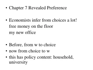
Chapter 7 Revealed Preference
Chapter 7 Revealed Preference Before, from w to choice, now from choice to a rational preference w (this has policy content: household, university) Some maintained assumptions A1: The consumer’s preferences are stable over the time period for which we observe his/her choice behaviors.

Chapter 7 Revealed Preference
E N D
Presentation Transcript
Chapter 7 Revealed Preference • Before, from w to choice, now from choice to a rational preference w (this has policy content: household, university) • Some maintained assumptions • A1: The consumer’s preferences are stable over the time period for which we observe his/her choice behaviors. • A2: There exists a unique demanded bundle for each budget set (strict convexity).
Def: If (x1, x2) is chosen at (p1, p2, m), (y1, y2)≠ (x1, x2) and p1y1+p2 y2≤m, then (x1, x2) is directly revealed preferred to (y1, y2). Denote this by (x1, x2) d (y1, y2). • Note that revealed preferred is solely about choices though choices are related to preferences. • A3: The consumer is always choosing the best s\he can afford (model of behavior).
From revealed preference (d) to preference (w): Suppose (x1, x2) is directly revealed preferred to (y1, y2) and the consumer is choosing the best s\he can afford, then (x1, x2) s (y1, y2). • Def: If (x1, x2) d (y1, y2) and (y1, y2) d (z1, z2), then we say that (x1, x2) is indirectly revealed preferred to (z1, z2). Denote this by (x1, x2) id (z1, z2). Allow indirect revealed preference for “chains” of observed choices longer than 3.
Def: If either (x1, x2) d (y1, y2) or (x1, x2) id (y1, y2), we say (x1, x2) is revealed preferred to (y1, y2). Denote this by (x1, x2) r (y1, y2). • Give an example to recover preferences. • We now question A3 (the idea is A1 and A2 are OK). How do we know whether the consumer is maximizing if we only observe choices?
The weak axiom of revealed preference (WARP): if (x1, x2) d (y1, y2), then it cannot happen that (y1, y2) d (x1, x2). (draw) (WARP is a weak and logical implication of consumers’ maximizing behaviors) • An example:
The strong axiom of revealed preference (SARP): if (x1, x2) r (y1, y2) and (x1, x2)≠ (y1, y2), then it cannot happen that (y1, y2) r (x1, x2). (SARP is a necessary and sufficient condition for optimizing behavior, but the proof is beyond the scope of this course.) (If choices satisfy SARP, then we can construct preferences for which the observed behavior is optimizing.)
Index numbers • Compare the consumption bundles of a consumer at two different times. Let b stand for the base period, t some other period. • At t: prices (p1t, p2t), consumption (x1t, x2t) • At b: prices (p1b, p2b), consumption (x1b, x2b)
Quantity index: compare the average consumption of these two periods, naturally could use the prices to be the weights • Laspeyres quantity index (use base price): Lq=(p1b x1t + p2b x2t)/(p1b x1b + p2b x2b), if Lq<1, at base price, base is chosen over t, so better off at base than at t (Lq>1?) • Paasche quantity index (use t price): Pq=(p1t x1t + p2t x2t)/(p1t x1b + p2t x2b), if Pq>1, at t price, t is chosen over base, so better off at t than at base (Pq<1?)
Price index: compare the average price of these two periods, naturally could use the quantities to be the weights • Laspeyres price index (use base q): Lp=(p1t x1b + p2t x2b)/(p1b x1b + p2b x2b), if Lp<1 (says nothing since prices different) • Paasche price index (use t q): Pp=(p1t x1t + p2t x2t)/(p1b x1t + p2b x2t)
Define a new index of the change in total expenditure M=(p1t x1t + p2t x2t)/(p1b x1b + p2b x2b). • Lp<M: p1t x1b + p2t x2b <p1t x1t + p2t x2t, t period is better than base (intuitively, when income grows faster than prices, better off after this change) • Pp>M: p1b x1b + p2b x2b> p1b x1t + p2b x2t, base is better than t (intuitively, when prices grow faster than income, worse off)
Social security: indexing so that base consumption is still affordable, then t cannot be worse than base