Download
1 / 14
140 likes | 320 Views
Testing seasonal adjustment with Demetra+. Dovnar Olga Alexandrovna The National Statistical Committee, Republic of Belarus. Check the original time series.

E N D
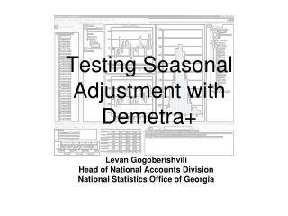
Testing seasonal adjustment with Demetra+ Dovnar Olga AlexandrovnaThe National Statistical Committee, Republic of Belarus
Check the original time series This report presents the results of the seasonal adjustment of time series of the index of industrial production of the Republic of Belarus Conclusions about the quality of source data Original time series is a monthly index of industrial production with base year 2005 Length of time series is 72 observations (1.2005-12.2010) In 2011, the statistical classification NACE/ISIC rev.3 was introduced into the practice of the Republic of Belarus. In this regard, this time series of indices of industrial production by NACE was obtained not by processing raw data, but by recalculating the structure of previously existing series of monthly indices based on the previous classification. The quality of the series received in that way Belstat considers not sufficiently precise, but quite satisfactory for statistical analysis, as the proportion of data relating to the industry by NCES is 98% of the total industrial output by NACE. In process of receipt of the new observations based on NACE, the quality of the time series will be improved.
The presence of seasonality in the original series Fig. 1 In the original time series a seasonal factor is present, what is indicated by the presence of spectral peaks at seasonal frequencies, and calendar effects.
Approach and predictors The approach TRAMO/SEATS was used User-defined specification TramoSeatsSpec-1 was used:
Pre-treatment The estimated period: [1-2005 : 12-2010] Logarithmically transformed series was chosen. Calendar effects (2 variables: the working days, a leap year).No effects of Easter. Type of used model is ARIMA model [(0,1,1)(0,1,1)].. Deviating values: identified one deviating value in November.
Graph of results Fig. 2 Seasonal component in the irregular component is not lost
Decomposition The basic model ARIMA of the time series of industrial production indices of the Republic of Belarus : (1-0,34В)(1 - 0,25 B12)at, σ2 = 1, decomposed into three sub-models: Trend model: (1 + 0,1B - 0,9B2)ap,t., σ2 = 0,0334 Seasonal model: (1 + 1,43B + 1,51B2 + 1,45 B3 + 1,25B4 + 1,01B5 + 0,74B6 + +0,47B7 + 0,24B8 + 0,03B9 + 0,11B10 - 0,40B11)as,t, σ2 = 0,1476 Irregular model: white noise(0; 0,1954). Dispersion of seasonal and trend components are lower than the irregular component. This means that stable trend and seasonal components were obtained.
Stability of the model The graphs of seasonally adjusted series (SA, Fig. 4) and trend (Fig. 5) shows that the updates are insignificant. The model can be considered as stable, because the difference between the first and the last estimates does not exceed 3%. There is one value on the graph of the Trend, exceeding the critical limit (March 2010 = 1.976). Seasonally adjusted series (SA) Trend Fig. 4 Fig. 5 Mean=0,3792 rmse=0.6888 Mean=0,3792 rmse=0.6888
Analysis of the residuals Fig. 6 The test results shows that residuals are independent, random and normal. Tests for nonlinearity did not show non-linearity in the form of trends.
Residual seasonal factor Fig. 7 We can assume that there are no indicators of residual seasonal fluctuations in the residues. But there is one peak at the small spectral seasonal frequency and one at the frequency of operating days, which may mean that the used filters are not the best to remove them.
Some problematic results How to connect the national calendar of holidays when applying built-in specs? The curve of the seasonality graph has not a visually clear structure (Fig. 8). How to interpret this? When using the model ARIMA model (0, 1, 0)(1, 0, 0) a purple line appeared on the chart (Fig. 9). What does it mean? What does the lack of graphs in the autoregressive spectrum of the spectral analysis of residuals mean? Is it a problem if there are small spectral peaks in the periodogram? (Fig. 7, slide 12). Fig. 8 Fig. 9
Some problematic results (continued) 5.How to correctly interpret a situation where innovation variance of the irregular component is lower than the trend and seasonality when using the ARIMA (0,1,0)(1, 0, 0) model? trend. Innovation variance = 0,0821 seasonal. Innovation variance = 0,1989 irregular. Innovation variance = 0,0971 6. Is it a problem if there is hypothetical autocorrelation in the seasonally adjusted series of lag 6, with using the ARIMA (0,1,1)(0, 1, 1) model? Autocorrelation functionseasonal : 7. Can they be considered as acceptable results of the Ljung-Boxand Box-Pierce tests for the presence of seasonality in residuals at lags 24 and 36 when using ARIMA (0,1,0) (1, 0, 0), or does it mean not using a suitable model?