Download

1 / 30
300 likes | 560 Views
Isosurface Extraction and Spatial Filtering Using Persistent Octree (POT). Qingmin Shi and Joseph JaJa Institute for Advanced Computer Studies and Department of Electrical and Computer Engineering University of Maryland, College Park. Volumetric Data Visualization. NLM Visible Human

E N D
Isosurface Extraction and Spatial Filtering Using Persistent Octree (POT) Qingmin Shi and Joseph JaJa Institute for Advanced Computer Studies and Department of Electrical and Computer Engineering University of Maryland, College Park
Volumetric Data Visualization NLM Visible Human ([Lorensen Vis’95]) LLNL Richtmyer-Meshkov Instability ([Shi, JaJa Vis’06]) Tetra Meshes of Ribosome 30S ([Zhang, Xu, and Bajaj, Computer Aided Geometric Design 2006])
Elevation Map: 2D-contours, each with a constant elevation Isosurface Extraction and Rendering • What is isosurface? Isosurface: A 3D-contour -- A 2D-surface embedded in a 3D space with constant density (isovalue) C. Image created from the UNC CT Head data set using VolPack [Lacroute and Levoy, SIGGRAPH ’94].
Basic Steps in Isosurface Computation • Finding the active cells that are cut by the isosurface. • Piece-wise linear approximation (triangulation) of the isosurface patches in each active cell. • The marching cubes algorithm was used in this paper. • Rendering triangles using either hardware or software.
Identifying Active Cells • Why is this step important? • Volume size can be very large. • The size of the whole Richtmyer-Meshkov instability data set is about 2.1 TB! • The isosurface in general only occupies a small subspace. • Examining all cells is very expensive and unnecessary. • Solution: value based partitioning.
Active Cell Identification As A Stabbing Query • Let miniandmaxibe the minimum and maximum scalar value of all the vertices of a cell i. • A cell is active if and only if the isovalue C is within the range [mini, maxi]. • Finding active cells is equivalent to stabbing a set of horizontal segments with an infinite vertical line. C
Solutions to the Stabbing Query • Optimal solutions: • Priority tree (McCreight SIAM J. Comp.’85). • Interval tree (Cignoni et al. Volvis’96, Chiang and Silva Vis’97). • Space: O(N), query time: O(log N + K) N: number of cells; K: number of active cells. • Good practical solutions • Span space (Livnat, Shen, Johnson Vis’96). • Span triangles (von Rymon-Lipinski et al. Vis’04). • Fixed-sized buckets (Waters, Co, and Joy EuroVis’05).
Spatial Filtering • Only a subset of the active cells need to be processed: • View-dependent rendering – cells that are visible. • Ray casting – the first active cell that intersects each ray. • 4D isosurface visualization – cells that intersect the cutting hyperplane. • Benefits: • Reduced indexing structure search time. • Reduced triangulation time. • Reduced rendering time.
View-dependent Isosurface Rendering • Render the isosurface patches in a front-to-back order. • Keep a coverage mask to tell which part of the screen has been covered. • Do not triangulate and render active cells whose projection to the screen has already been covered. Problem: How to examine the active cells in a front-to-back order?
Value-based vs. Location-based Partitioning • Previous view-dependent algorithms often employ location-based partitioning. • Example: a min-max octree equipped with min, max values for each internal node. • Problem: identifying active cells is inefficient. • Active cells reported by a value-based partitioning structure do not obey any spatial ordering.
Our Solution • Build one octree to organize the active cells corresponding to EACH possible isovalue. • Compress the sequence of octrees into a persistent octree (POT). • The benefits of both approaches: • The size of the POT is linear in the input size O(N), even for continuous data types! • Identifying visible active cells is done by a front-to-back traversal of an octree that consists of ONLY the active cells – O(K)! • Spatial filtering is efficient using the octree.
Version 2 of D Persistent Data Structures • Consider a dynamic data structure D. • Each insertion/deletion produces a new version of D. • The entire evolution history of D is recorded as P. • Any particular version of D can be searched by knowing its version number. • If the cost of each update is small, the entire persistent data structure is small. D(0) D(2) D(3) D(1) A persistent data structure P
isovalue sweeping line Handling Stabbing Queries Using Persistent Data Structures S1 S2 S3 S4 S5 scalar value V0 V1 V2 V3 V5 V6 V7 V8 V9 V10 V4
A Standard Octree • Orange nodes represent active cells (regions). • Gray nodes represent mixed regions. • White (non-active) nodes can be omitted. • Not suitable to be made persistent. • Why? A single update operation requires significant change of the data structure.
The Compact Octree • What’s good about the compact octree? On average, only a CONSTANT number of changes need to be made to the tree. • So? The corresponding persistent octree requires LINEAR space.
insert insert insert Update the Compact Octree – The Insertion Case 2: Case 1: Case 3:
Case 2: Case 1: Case 3: Update the Compact Octree – The Deletion An expensive delete operation. Fortunately, it does not happen very often. Amortized update complexity: still O(1). Not true for arbitrary delete/insert operation.
System Setup • A Linux PC with dual Xeon 3.0 GHz processors (only one was used). • 8 GB memory. • 150 GB local disk. • NVidia6800 Ultra GPU card.
Data Sets • Downsampled LLNL Richtmyer-Meshkov Instability Data Set (byte, 1024 x 1024 x 960 x 35 time steps). • Stanford Bunny (short, 512 x 512 x 360). • UNC MR Brain (short, 256 x 256 x 109). • Head Aneurysm (byte 512 x 512 x 512) (Michael Meißner, Viatronix Inc., USA).
Storage Cost# The POT is about 1.6 to 4 times bigger. # Both BONO and POT are built on 4x4x4 cell blocks. * The above table only lists the sizes of the indexing structures. The sizes of the raw data sets are the same for both BONO and POT and thus are omitted here. + [Wilhelms and Van Gelder, ACM Trans. on Graphics, 92].
Performance Comparison of View-independent Isosurface Extraction
Performance Comparison of View-dependent Isosurface Extraction
Other Applications of POT • Isosurface rendering by Ray-casting. • Go straight to the intersecting active cell. • Rendering time-varying data (4-D isosurface) • A 4-D isosurface can only be visualized by slicing it using a 4-D hyperplane. • POT can be used to quickly identify cells that are both active and relevant (cut by the hyperplane). • Multi-resolution isosurface rendering • Triangulate supercells at different resolutions. • Internal nodes in a POT naturally represent active supercells.
Conclusions • Good things about POT. • Simultaneous pruning in both value and viewing space. • Fast search time and reasonable storage cost. • Hierarchical organization of active cells facilitates spatial search. • Further improvements. • Need tests on continuous data types. • Improve the search time and storage cost. • How to incorporate this technique into parallel/distributed isosurface rendering systems.
Thank You! Questions?
Isosurfacing By Ray Casting • The basic scheme: • Shoot a ray from each pixel towards the volume. • Identify the foremost active cell intersected by the ray. • Analytically compute the position of the intersection point. • Shade the intersection point. • The bottle neck: traversal of non-active cells. • Using POT: • No active cells in the octree. • No need to examine non-active regions. • An example: • Standard ray-casting: 9 cells to examine. • POT: 3 nodes to visit.
An Example of VD Isosurfacing A front view of the MRI Head The side view The final coverage mask
More Pictures A top view of the MRI-brain data Stanford bunny Cutting plane: X=500 Cutting plane: Z=650
Practical Issues • Build POT on 4x4x4 cubes rather than individual cells. • Sequentialize the POT (an acyclic graph) on disk. • Use hierarchical coverage mask to speedup visibility test (Greene SIGGRAPH’96, Livnat and Hansen Vis’98).