Download
1 / 79
790 likes | 961 Views
The Dynamics of Attending and Scene Analysis. By Mari Riess Jones. Thanks to . Ralph Barnes Devin McAuley Heather Moynihan Noah MacKenzie Amandine Penel Jennifer Puente Nate Vaughan. Special Thanks to Edward Large. Overview.

E N D
The Dynamics of Attending andScene Analysis By Mari Riess Jones
Thanks to Ralph Barnes Devin McAuley Heather Moynihan Noah MacKenzie Amandine Penel Jennifer Puente Nate Vaughan Special Thanks to Edward Large
Overview • Scene Analysis: A Neo Gestalt view • Scene Analysis: A dynamic perspective • The Changing Scene: Tracking in real time
What’s a Scene? The term scene is taken from vision. Two cases are most common: 1. A stationary viewer 2. A moving viewer The scene is the static visual layout.
Sound Scenes A common assumption: We use the proximal sound stimulus to recover the location and/or identity of a distal, vibrating, object within a scene. This is the source identity principle.
Bregman’s Theoryof Scene Analysis Bregman builds on this idea: Goal of auditory perception… is identification of one or more sources of a proximal mixture of sounds. If an unfolding sound pattern is perceived as a structurally intact , i.e. as one stream, then it must come from ONE source.
Other patterns? Patterns NOT perceived as intact…. If a pattern is perceived to break up, i.e. form N different subjective units, streams, then, it must … come from N separate sources.
Example: A sound pattern Another source? high A stream ? frequency One source? low Time
The Big Question What makes a pattern seem structurally intact? Or… What determines a stream?
Bregman’s Answer Involves a two stage theory in which Neo Gestalt principles are critical.
The Neo Gestalt View Two Stages • Primitive processesInnate, automatic, effortless, Determine coherent perceptual groups at fast rates. • II. Schema driven processesLearned, voluntary, effortful, Determine attention to groupings at slow rates.
Auditory Scene Perception Stage I: Primitive Processes Operate on Gestalt grouping principles: proximity in frequency and time; similarity (e.g., timbre); continuity; exclusive allocation… and so forth These are domain general (I.e. speech, music, natural environs,etc.)
Proximity vs Continuity Tougas and Bregman (1985) In a series of famous studies pitted proximity against continuity. Goal:To assess which principle dominated, and to dispute a trajectory explanation. Bouncing versus Crossing trajectories
Possible Percepts Time in seconds
Conclusion People hear bouncing patterns Proximity in frequency dominates
Rhythm Perception A stream usually conveys a rhythm Speeding up a sequence can break it , perceptually, into interleaved streams This changes its perceived rhythm!
Rhythm Rhythm perception… depends on the relationship of frequency change (f )to time change (t). Hi frequency t 2 t f Lo frequency Time This slow melody… is perceived to have a ‘galloping ‘rhythm
But… That Rhythm Disappears In a faster melody with the same tones. Now we hear two melodies (streams) each with anisochronousrhythm.
A Neo Gestalt Explanation • Builds on Gestalt proximity: • Temporal proximity is heightened at fast rates. • But frequency proximity dominates. • Two streams form based on pitch proximity: A high tone stream and a low tone stream.
Auditory Patterns Most of our environment comprises sources that turn on and off and modulate over time to project pattern structure that is…. motion-like and rhythmic
Important Pattern Properties • Motionlike properties: Rates of change. • [ e.g., f/t ] 2. Rhythmic properties:Relative timing. [e.g., ti/tk ]
Motionlike Trajectories In 1976, I proposed that the rate-of-change of frequency (log scale) may be perceived as a sort of velocity. Pitch Velocity: f / t
Determinants of Pitch Velocity high f frequency f/ t t low Time A sudden increase in rate-of-change in an isochronous rhythm is perturbing.
Motionlike Trajectory limits on pitch velocity? LARGE streamed Intact Serial Percepts Velocity Limit f log Stimulus patterns SMALL FAST t Slow RATE (Jones, 1976)
Rhythmic Properties: Relative Timing Limit Slower patterns flog FAST t =IOI SLOW RATE
Alternative View: A focus on time How do rhythmic properties of a pattern affect real time responding to it? In the remainder of this talk, I address this question.
General Assumptions Environment Scenes often project dynamic patterns with relative timing that is quasi- periodic. Living things Animate creatures possess internal periodicities that can synchronize to patterns. Connecting through time Pattern timing determines how living things connect with a changing scene.
Some quasi-periodic patterns t = IOI = 700 ms Great Gray Owl Horned Lark Cardinal
Internal Periodicities: Biological Oscillations Many internal periodicities exist; periods of 1 ms, several minutes, years !. Most studied are circadian rhythms; oscillatory periods of ca. 24 hours.
Connecting “How do internal oscillations of an organism connect with pattern timing? “ One answer: By synchronizing. More precisely: By entrainment
Biological Entrainment Pittendrigh & Daan (1976) . Circadian rhythms of 24 hours synchronize to light/dark cycles. Daan et al. (2001) recently updated this two oscillator model.
Example: Two Entraining Oscillations Winter M Phase locked E Phase locked Summer From Daan et al. J.Biological Rhythms (2001)
Shorter Periods? In species with refined use of fast sound patterns, Can we postulate, internal oscillations with periods less than the circadian period ?
Generalizing….. Alternatively Other Oscillators Most Biological Oscillators Long natural periods Respond to light changes Short natural periods Respond to sound changes
Background:Rhythmic (periodic) Expectancies Quasi-periodicities in Rhythmical sound patterns Induce Periodic expectancies Perhaps such expectancies reflect entrainments to patterns of stimulus IOIs?
Back to Synchrony: Asimple premise When we attend , an internal activity is elicited … that co-occurs with the attended object. This activity involves Internal oscillations (Jones, 1976).
Attending to Dynamic Patterns Where elements appear… then disappear Time Attention must occur in synchrony with elements.
Dynamic Attending Postulates that : Selective attending in time is paced by stimulus timing. Attentional focus in time becomes phase-locked to elements.
Attending oscillates in time Resources are periodically distributed as internal oscillations. Inter-onset-interval, IOI Time Pulses of attention energy
Formalized as an Oscillator Model : by Ed Large (Large & Jones, 1999) Stimulus IOI Expected point in time Phase Period Periodic Expectancies Stimulus timing paces the oscillator. Oscillator period and phase determine this entrainment .
The adaptive oscillator Tones, i Period, Pi Phase, i Period and Phase change: They draw attending rhythms to “fit” a time pattern. Period changes Phase changes
A simple dynamical system. The entrained oscillator gravitates to an attractor state of: • 1. Phase Synchrony:A zero time difference between an sound onset and a pulse peak. • 2. Period matching:A zero time difference between an IOI and oscillator period (limit cycle).
Relative Phase, i Gives observed - expected times i is the order variable in this system. It summarizes the state of the system at any instant i. i+1 = i + IOIi+1/Pi - F(i) The coupling term, F, here is sinusoidal: F()= {1/2}sin 2 =>
Theoretical Entrainment Region { = 1.0 } - Phase Attractor: Synchrony Phase Attractor:synchrony .25 .25 -.25 -.25 Relative Phase, i
What does this approach purchase ? A few experiments….
Preview: Our Experimental Designs Will involve a context rhythm, given by tones: C Followed by a comparison, C, (of some sort) Time JudgmentComparison IOI Pitch JudgmentComparison tone
Time Judgment TasksRationale If relative timing in sound arrays entrains attending, then the context rhythm should Shape temporal expectancies Affect time judgments.