Download

1 / 67
730 likes | 979 Views
Nanomaterials. Boxuan Gu and David McQuilling. What are they?. Nano = 10 -9 or one billionth in size Materials with dimensions and tolerances in the range of 100 nm to 0.1 nm Metals, ceramics, polymeric materials, or composite materials One nanometer spans 3-5 atoms lined up in a row

E N D
Nanomaterials Boxuan Gu and David McQuilling
What are they? • Nano = 10-9 or one billionth in size • Materials with dimensions and tolerances in the range of 100 nm to 0.1 nm • Metals, ceramics, polymeric materials, or composite materials • One nanometer spans 3-5 atoms lined up in a row • Human hair is five orders of magnitude larger than nanomaterials
Nanomaterial Composition • Comprised of many different elements such as carbons and metals • Combinations of elements can make up nanomaterial grains such as titanium carbide and zinc sulfide • Allows construction of new materials such as C60 (Bucky Balls or fullerenes) and nanotubes
How they are made • Clay/polymer nanocomposites can be made by subjecting clay to ion exchange and then mixing it with polymer melts • Fullerenes can be made by vaporizing carbon within a gas medium • Current carbon fullerenes are in the gaseous phase although samples of solid state fullerenes have been found in nature
Bucky Ball properties • Arranged in pentagons and hexagons • A one atom thick seperation of two spaces; inside the ball and outside • Highest tensile strength of any known 2D structure or element, including cross-section of diamonds which have the highest tensile strength of all known 3D structures (which is also a formation of carbon atoms) • Also has the highest packing density of all known structures (including diamonds) • Impenetrable to all elements under normal circumstances, even a helium atom with an energy of 5eV (electron Volt)
Bucky Ball properties cont. • Even though each carbon atom is only bonded with three other carbons (they are most happy with four bonds) in a fullerene, dangling a single carbon atom next to the structure will not affect the structure, i.e. the bond made with the dangling carbon is not strong enough to break the structure of the fullerene • No other element has such wonderful properties as carbon which allows costs to be relatively cheap; after all it’s just carbon and carbon is everywhere
Buckminsterfullerene uses • Due to their extremely resilient and sturdy nature bucky balls are debated for use in combat armor • Bucky balls have been shown to be impervious to lasers, allowing for defenses from future warfare • Bucky balls have also been shown to be useful at fighting the HIV virus that leads to AIDS • Researchers Kenyan and Wudl found that water soluble derivates of C60 inhibit the HIV-1 protease, the enzyme responsible for the development of the virus • Elements can be bonded with the bucky ball to create more diverse materials including superconductors and insulators • Can be used to fashion nanotubes
Bucky Balls C240 colliding with C60 at 300 eV (Kinetic energy) Bucky Ball (C60) http://www.pa.msu.edu/cmp/csc/simindex.html
Nanotube properties • Superior stiffness and strength to all other materials • Extraordinary electric properties • Reported to be thermally stable in a vacuum up to 2800 degrees Centigrade (and we fret over CPU temps over 50o C) • Capacity to carry an electric current 1000 times better than copper wires • Twice the thermal conductivity of diamonds • Pressing or stretching nanotubes can change their electrical properties by changing the quantum states of the electrons in the carbon bonds • They are either conducting or semi-conducting depending on the their structure
Nanotube uses • Can be used for containers to hold various materials on the nano-scale level • Due to their exceptional electrical properties, nanotubes have a potential for use in everyday electronics such as televisions and computers to more complex uses like aerospace materials and circuits
Nanotubes Switching nanotube-based memory Carbon based nanotubes http://www.pa.msu.edu/cmp/csc/simindex.html
Applications of Nanotechnology • Next-generation computer chips • Ultra-high purity materials, enhanced thermal conductivity and longer lasting nanocrystalline materials • Kinetic Energy penetrators (DoD weapon) • Nanocrystalline tungsten heavy alloy to replace radioactive depleted uranium • Better insulation materials • Create foam-like structures called ‘aerogels’ from nanocrystalline materials • Porous and extremely lightweight, can hold up to 100 times their weight
More applications… • Improved HDTV and LCD monitors • Nanocrystalline selenide, zinc sulfide, cadmium sulfide, and lead telluride to replace current phosphors • Cheaper and more durable • Harder and more durable cutting materials • Tungsten carbide, tantalum carbide, and titanium carbide • Much more wear-resistant and corrosion-resistant than conventional materials • Reduces time needed to manufacture parts, cheaper manufacturing
Even more applications… • High power magnets • Nanocrystalline yttrium-samarium-cobalt grains possess unusually large surface area compared to traditional magnet materials • Allows for much higher magnetization values • Possibility for quieter submarines, ultra-sensitive analyzing devices, magnetic resonance imaging (MRI) or automobile alternators to name a few • Pollution clean up materials • Engineered to be chemically reactive to carbon monoxide and nitrous oxide • More efficient pollution controls and cleanup
Still more applications… • Greater fuel efficiency for cars • Improved spark plug materials, ‘railplug’ • Stronger bio-based plastics • Bio-based plastics made from plant oils lack sufficient structural strength to be useful • Merge nanomaterials such as clays, fibers and tubes with bio-based plastics to enhance strength and durability • Allows for stronger, more environment friendly materials to construct cars, space shuttles and a myriad of other products
Applications wrapup • Higher quality medical implants • Current micro-scale implants aren’t porous enough for tissue to penetrate and adapt to • Nano-scale materials not only enhance durability and strength of implants but also allow tissue cells to adapt more readily • Home pregnancy tests • Current tests such as ‘First Response’ use gold nanoparticles in conjunction with micro-meter sized latex particles • Derived with antibodies to the human chorionic gonadotrophin hormone that is released by pregnant women • The antibodies react with the hormone in urine and clump together and show up pink due to the nanoparticles’ plamson resonance absortion qualities
Modeling and Simulation of Nanostructured Materials and Systems
Preface • Each distinct age in the development of humankind has been associated with advances in materials technology. • Historians have linked key technological and societal events with the materials technology that was prevalent during the “stone age,” “bronze age,” and so forth.
Significant events In materials • 1665 - Robert Hooke …material microstructure • 1808 - John Dalton … atomic theory • 1824 - Portland cement • 1839 - Vulcanization • 1856 - Large-scale steel production • 1869 - Mendeleev and Meyer … Periodic Table of the Chemical Elements • 1886 - Aluminum • 1900 - Max Planck …. quantum mechanics
Cont. • 1909 - Bakelite • 1921 - A. A. Griffith …. fracture strength • 1928 - Staudinger… polymers (small molecules that link to form chains) • 1955 - Synthetic diamond • 1970 - Optical fibers • 1985 - First university initiatives attempt computational materials design • 1985 - Bucky balls (C60) discovered at Rice University • 1991 - Carbon nanotubes discovered by Sumio Iijima
Why we need Computational Materials? Traditionally, research institutions have relied on a discipline-oriented approach to material development and design with new materials. It is recognized, however, that within the scope of materials and structures research, the breadth of length and time scales may range more than 12 orders of magnitude, and different scientific and engineering disciplines are involved at each level.
To help address this wide-ranging interdisciplinary research, Computational Materials has been formulated with the specific goal of exploiting the tremendous physical and mechanical properties of new nano-materials by understanding materials at atomic, molecular, and supramolecular levels.
Computational Materials at LaRC draws from physics and chemistry, but focuses on constitutive descriptions of materials that are useful in formulating macroscopic models of material performance.
Benefit of Computational materials • First, it encourages a reduced reliance on costly trial and error, or serendipity, of the “Edisonian” approach to materials research. • Second, it increases the confidence that new materials will possess the desired properties when scaled up from the laboratory level, so that lead-time for the introduction of new technologies is reduced. • Third, the Computational Materials approach lowers the likelihood of conservative or compromised designs that might have resulted from reliance on less-than-perfect materials.
Schematic illustration of relationships between time and length scales for the multi-scale simulation methodology.
Cont. • The starting point is a quantum description of materials; this is carried forward to an atomistic scale for initial model development. Models at this scale are based on molecular mechanics or molecular dynamics.
Cont. • At the next scale, the models can incorporate micro-scale features and simplified constitutive relationships. • Further progress up, the scale leads to the meso or in-between levels that rely on combinations of micromechanics and wellestablished theories such as elasticity.
Cont. • The last step towards engineering-level performance is to move from mechanics of materials to structural mechanics by using methods that rely on empirical data,constitutive models, and fundamental mechanics.
Nanostructured Materials • The origins of focused research into nanostructured materials can be traced back to a seminal lecture given by Richard Feynman in 1959[1]. • In this lecture, he proposed an approach to “the problem of manipulating and controlling things on a small scale.” The scale he referred to was not the microscopic scale that was familiar to scientists of the day but the unexplored atomistic scale.
The nanostructured materials based on carbon nanotubes and related carbon structures are of current interest for much of the materials community. • More broadly then, nanotechnology presents the vision of working at the molecular level, atom by atom, to create large structures with fundamentally new molecular organization.
Atomistic, Molecular Methods • The approach taken by the Computational Materials is formulation of a set of integrated predictive models that bridge the time and length scales associated with material behavior from the nano through the meso scale.
At the atomistic or molecular level, the reliance is on molecular mechanics, • molecular dynamics, and coarse-grained, Monte-Carlo simulation. • Molecular models encompassing thousands and perhaps millions of atoms can be solved by these methods and used to predict fundamental, molecular level material behavior. The methods are both static and dynamic.
Molecular dynamics simulations generate information at the nano-level, including atomic positions and velocities. • The conversion of this information to macroscopic observables such as pressure, energy, heat capacities, etc., requires statistical mechanics.
An experiment is usually made on a macroscopic sample that contains an extremely large number of atoms or molecules, representing an enormous number of conformations. • In statistical mechanics, averages corresponding to experimental measurements are defined in terms of ensemble averages.
For example where M is the number of configurations in the molecular dynamics trajectory and Vi is the potential energy of each configuration.
where M is the number of configurations in the simulation, N is the number of atoms in the system, mi is the mass of the particle i and vi is the velocity of particle i. To ensure a proper average, a molecular dynamics simulation must account for a large number of representative conformations.
By using Newton’s second law to calculate a trajectory, one only needs the initial positions of the atoms, an initial distribution of velocities and the acceleration, which is determined by the gradient of the potential energy function. • The equations of motion are deterministic; i.e., the positions and the velocities at time zero determine the positions and velocities at all other times, t. In some systems, the initial positions can be obtained from experimentally determined structures.
In a molecular dynamics simulation, the time dependent behavior of the molecular system is obtained by integrating Newton’s equations of motion. • The result of the simulation is a time series of conformations or the path followed by each atom. • Most molecular dynamics simulations are performed under conditions of constant number of atoms, volume, and energy (N,V,E) or constant number of atoms, temperature, and pressure (N,T,P) to better simulate experimental conditions.
Basic steps in the MD simulation • 1. Establish initial coordinates. • 2. Minimize the structure. • 3. Assign initial velocities. • 4. Establish heating dynamics. • 5. Perform equilibration dynamics. • 6. Rescale the velocities and check if the temperature is correct. • 7. Perform dynamic analysis of trajectories.
Monte Carlo Simulation • Although molecular dynamics methods provide the kind of detail necessary to resolve molecular structure and localized interactions, this fidelity comes with a price. Namely, both the size and time scales of the model are limited by numerical and computational boundaries.
To help overcome these limitations,coarse-grained methods are available that represent molecular chains as simpler, bead-spring models. • Coarse-grain models are often linked to Monte Carlo (MC) simulations to provide a timely solution. • The MC method is used to simulate stochastic events and provide statistical approaches to numerical Integration.
There are three characteristic steps in the MC simulation that are given as follows. 1. Translate the physical problem into an analogous probabilistic or statistical model. 2. Solve the probabilistic model by a numerical sampling experiment. 3. Analyze the resultant data by using statistical methods.
Continum Methods • Despite the importance of understanding the molecular structure and nature of materials, at some level in the multi-scale analysis the behaviour of collections of molecules and atoms can be homogenized.
At this level, the continuum level, the observed macroscopic behaviour is explained by disregarding the discrete atomistic and molecular structure and assuming that the material is continuously distributed throughout its volume. The continuum material is assumed to have an average density and can be subjected to body forces such as gravity and surface forces such as the contact between two bodies.
The continuum can be assumed to obey several fundamental laws. • The first, continuity, is derived from the conservation of mass. • The second, equilibrium, is derived from momentum considerations and Newton’s second law. • The third, the moment of momentum principle, is based on the model that the time rate of change of angular momentum with respect to an arbitrary point is equal to the resultant moment.
These laws provide the basis for the continuum model and must be coupled with the appropriate constitutive equations and equations of state to provide all the equations necessary for solving a continuum problem. • The state of the continuum system is described by several thermodynamic and kinematic state variables. • The equations of state provide the relationships between the non-independent state variables.
The continuum method relates the deformation of a continuous medium to the external forces acting on the medium and the resulting internal stress and strain. • Computational approaches range from simple closed-form analytical expressions to micromechanics to complex structural mechanics calculations basedon beam and shell theory.
The continuum-mechanics methods rely on describing the geometry, (I.e.physical model), and must have a constitutive relationship to achieve a solution. • For a displacement –based form of continuum solution, the principle of virtual work is assumed valid.