Bayesian Quantum Tomography
Bayesian Quantum Tomography. Byron Smith December 11, 2013. Outline. What is Quantum State Tomography? What is Bayesian Statistics? Conditional Probabilities Bayes ’ Rule Frequentist vs. Bayesian Example: Schrodinger’s Cat Interpretation Analysis with a Non-informative Prior

Bayesian Quantum Tomography
E N D
Presentation Transcript
Bayesian Quantum Tomography Byron Smith December 11, 2013
Outline • What is Quantum State Tomography? • What is Bayesian Statistics? • Conditional Probabilities • Bayes’ Rule • Frequentist vs. Bayesian • Example: Schrodinger’s Cat • Interpretation • Analysis with a Non-informative Prior • Analysis with an Informative Prior • Sources of Error in Tomography • Error Reduction via Bayesian Analysis • Adaptive Tomography • Conclusion • References • Supplementary Information
What is Quantum (State) Tomography? • Tomography comes from tomos meaning section. • Classically, tomography refers to analyzing a 3-dimensional trajectory using 2-dimensional slices. • Quantum State Tomography refers to identifying a particular wave function using a series of measurements.
Bayes’ Rule is the Likelihood is the Prior Probability (or just prior) is the Posterior Probability (or just posterior)
Frequentist vs. Bayesian • Inference on probability arises from the frequency that some outcome is measured and that measurement is random. • In other words, a measurement is random only due to our ignorance. • Inference on probability arises from a prior probability assumption weighted by empirical evidence. • Measurements are inherently random. Frequentist Bayesian
Example: Interpretation of Schrodinger’s Cat Frequentist: Given N cats, there are some that are alive and some that are dead. The probability that the cat is alive is associated with the fact that we sample randomly and a*N of the cats are alive. Bayesian: The probability a is a random variable (unknown) and therefore there is an inherent probability associated with each particular cat.
A Graphical Comparison:Uniform Prior (α = 1, β= 1) True value of a = 0.3
A Graphical Comparison:Beta Prior (α = 3.1, β = 6.9) • Flourine-18, half-life=1.8295 Hours • Cat has been in for 3 hours
Sources of Error in Tomography • Error in the measurement basis. • Error in the counting statistics. • Error associated with stability. • Detector efficiency • Source intensity • Model Error
Estimation Error Frequentist Bayesian (α=3.1, β=6.9)
Density Estimation • There are several measures of “lack of fit.” • Likelihood • Infidelity • Shannon Entropy
Adaptive Tomography • The number of measurements required to sufficiently identify ρ can be reduced when using a basis which diagonalizesρ. • To do so, measure N0 particles first, change the measurement basis, then finish the total measurement. • Naturally this can be improved with Bayesian by using the first measurements as a Prior.
Conclusion • Quantum State Tomography is a tool used to identify a density matrix. • There are several metrics of density identification. • Bayesian statistics can improve efficiency while providing a new interpretation of quantum states.
References • J. B. Altepeter, D. F. V. James, and P. G. Kwiat, Qubit Quantum State Tomography, in Quantum State Estimation (Lecture Notes in Physics), M. Paris and J. Rehacek (editors), Springer (2004). • D. H. Mahler, L. A. Rozema, A. Darabi, C. Ferrie, R. Blume-Kohout, and A. M. Steinberg, Phys. Rev. Lett.111, 183601 (2013). • F. Huszár and N. M. T. Houlsby, Phys. Rev. A85, 052120 (2012). • R. Blume-Kohout, New J. Phys.12, 043034 (2012).
Stoke’s Parameters • For density operators which are not diagonal, we use a basis of spin matrices: • If choose an instrument orientation such that the first parameter is 1, we are left with the Stoke’s Parameters,Si: • The goal is then to identify the Si.
Poincare Spheres • Used to visualize a superposition of photon polarizations. • The x-axis is 45 degree polarizations. • The y-axis is horizontal or vertical polarizations. • The z-axis is circular polarizations.
Tomography with Poincare Spheres • Using a matrix basis similar to that for Stoke’s Parameters, one can exactly identify a polarization with three measurements. • Note that an orthogonal basis is not necessary.
Imperfect Tomogrpahy • Errors in measurement and instrumentation will manifest themselves as a disc on the Poincare Sphere: • (a) Errors in measurement basis. (b) Errors in intensity or detector stability.
Statistical Tomography • Because there is a finite sample size, states are not characterized exactly. • Each measurement constrains the sample space.
Pitfalls of Maximum Likelihood Analysis • Optimization can lead to states which lie outside the Poincare Sphere. • Unobserved values a registered as zeros in the density matrix optimization. This can be unrealistic. • There is no direct measure of uncertainty within maximum likelihood estimators.
Solutions through Bayesian Analysis • Parameter space can be constrained through the prior. • Unobserved values can still have some small probability through the prior. • Uncertainty analysis can come directly from the variance of the posterior distribution, regardless of an analytical form.