Download

1 / 33
340 likes | 494 Views
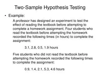
Hypothesis Testing-2 Sample. 8. Elementary Statistics Larson Farber. Section 8.1. Testing the Difference Between Two Means (Large Independent Samples). Overview.

E N D
Hypothesis Testing-2 Sample 8 Elementary Statistics Larson Farber
Section 8.1 Testing the Difference Between Two Means (Large Independent Samples)
Overview To test the effect of an herbal treatment on improvement of memory you randomly select two samples, one to receive the treatment and one to receive a placebo. Results of a memory test taken one month later are given. Sample 1 Sample 2 Experimental Group Treatment Control Group Placebo The resulting test statistic is 77 – 73 = 4. Is this difference significant or is it due to chance (sampling error)?
Independent Samples When members of one sample are not related to members of the other sample. Person’s receiving herbal treatment were not related or paired with those in the control group who took a placebo. x1 x1 x2 x2 x1 x2 x1 x1 x2 x1 x2 x1 Experimental Group Control Group
Dependent Samples Each member of one sample is paired with a member of the other sample. The test score for each person in the sample could be recorded before and after taking the herbal treatment. x1 x2 x1 x2 x1 x2 x1 x2 x1 x2 x1 x2 Score Before Score After The difference can be calculated for each pair.
Application To test the effect of an herbal treatment on improvement of memory, you randomly select a sample of 95 to receive the treatment and a sample of 105 to receive a placebo. Both groups take a test after one month. The mean score for the experimental group is 77 with a standard deviation of 15. For the control group, the mean is 73 with a standard deviation of 12. Test the claim that the herbal treatment improves memory at = 0.01.
1. Write the null and alternative hypothesis. Null Hypothesis H0 usually contains the equality condition. (There is no difference between the parameters of two populations.) Alternative Hypothesis Ha is true when H0 is false. Claim 2. State the level of significance. = 0.01. This is the probability that H0 is true, but you reject it.
3. Identify the sampling distribution. The distribution for the sample statistic is normal since both samples are large. Rejection Region z 0 2.33 Critical Value z0 z0 4. Find the critical value. 5. Find the rejection region.
When both samples are large, you can use s1 and s2 in place of and . 6. Find the test statistic. 7. Make your decision z 0 2.33 z = 2.07 does not fall in the rejection region. Do not reject the null hypothesis. The P-value is .019 >.01. Do not reject H0. 8. Interpret your decision. There is not enough evidence to support the claim that the herbal treatment improves memory.
Section 8.2 Testing the Difference Between Two Means (Small Independent Samples)
Testing Difference Between Means (Small Samples) When you cannot collect samples of 30 or more, you can use a t-test, provided both populations are normal. The sampling distribution depends on whether or not the population variances are equal. If the variances of the two populations are equal, you can combine or “pool” information from both samples to form a pooled estimate of the standard deviation. The standard error is d.f. = n1 + n2 - 2 If the variances are not equal, the standard error is: And d.f. is the smaller of n1 – 1 or n2 – 1.
Application 5 8 1520 937 403 382 Crash tests at 5 miles per hour were performed on 5 small pickups and 8 SUVs. For the small pickups the mean bumper repair cost was $1520 and the standard deviation was $403. For the SUVs the mean bumper repair cost was $937 and the standard deviation was $382. At = 0.05 test the claim that the bumper repair cost is greater for small pickups than for SUVs. Assume equal variances. Pickup SUV n s
Claim = 0.05. Since the variances are equal, the distribution for the sample statistic is a t-distribution with d.f. = 5 + 8 – 2 = 11. 1. Write the null and alternative hypothesis. 2. State the level of significance. 3. Identify the sampling distribution.
4. Find the critical value. 5. Find the rejection region t0 t 0 1.796 6. Find the test statistic. When variances are equal find the pooled value.
7. Make your decision. t 1.796 0 t = 2.624 falls in the rejection region. Reject the null hypothesis. 8. Interpret your decision. There is enough evidence to support the claim that bumper repair costs are greater for pickups than for SUVs.
Application A real estate agent claims there is no difference between the mean household incomes of two neighborhoods. The mean income of 12 households from the first neighborhood was $48,250 with a standard deviation of $1200. In the second neighborhood, 10 households has a mean income of $50,375 with a standard deviation of $3400. Assume the incomes are normally distributed and the variances are not equal. Test the claim at = 0.01.
12.000 10.000 48.250 50.375 1200.000 3400.000 1. Write the null and alternative hypothesis. First Second Claim n s 2. State the level of significance. . 3. Identify the sampling distribution. Since the variances are not equal, the distribution for the sample statistic is a t-distribution with d.f. = 9. (The smaller sample size is 10 and 10 - 1 = 9.)
4. Find the critical values. 5. Find the rejection regions. t0 –t0 0 t –3.250 3.250 6. Find the test statistic.
7. Make your decision. 0 t –3.250 3.250 t = –1.881 does not fall in the rejection region. Do not reject the null hypothesis. (The P-value is .087 > .01.) 8. Interpret your decision. There is not enough evidence to reject the claim that there is no difference in mean household incomes in the two neighborhoods.
Section 8.3 Testing the Difference Between Two Means (Dependent Samples)
The Difference Between Means-Dependent Samples When each value from one sample is paired with a data value in the second sample, the samples are dependent. x1 x2 x1 x2 x1 x2 x1 x2 x1 x2 x1 x2 The difference, d = x1 – x2 is calculated for each data pair. The sampling distribution for , the mean of the differences, is a t-distribution with n – 1 degrees of freedom. (n is the number of pairs.)
Application Person Before After d 1 65 127 62 2 72 135 63 3 85 140 55 4 78 136 58 5 93 150 57 The table shows the heart rates (beats per minute) of 5 people before exercising and after. Is there enough evidence to conclude that heart rate increases with exercise? Use . The mean of the differences d is 59 The standard deviation of d is 3.39
Claim The distribution for the sample statistic is a t-distribution with d.f. = 4. 1. Write the null and alternative hypothesis. 2. State the level of significance. 3. Identify the sampling distribution. (Since there are 5 data pairs, d.f.= 5 – 1 = 4.)
4. Find the critical value. 5. Find the rejection region. t0 0 t 2.132 6. Find the test statistic.
7. Make your decision. t0 0 t 2.132 t = 38.92 falls in the rejection region. Reject the null hypothesis. The P-value is very close to 0. 8. Interpret your decision. There is enough evidence to support the claim that heart rate increases with exercise.
Test of = 0.00 vs > 0.00 Variable diff. N 5 Mean 59.00 StDev 3.39 SE 1.52 Mean 5 T 38.90 P 0.0000 Using Minitab The Minitab printout The P-value is 0.0000. Since 0.0000 < 0.05, reject the null hypothesis.
Section 8.4 Testing the Difference Between Two Proportions
The Difference Between Proportions If independent samples are taken from each of two populations and the samples are large enough you can test for the difference between population proportions p1 – p2. x1 and x2 represent the number of successes in 1st and 2nd samples. n1 and n2 represent the total number in the 1st and 2nd samples. Sample proportions of successes. Since the proportions will be assumed equal, an estimate for the common value is:
the sampling distribution for is normal. and the standard error The standardized test statistic is: Two Sample z-Test If are each at least 5, The mean is p1 – p2 = 0
n2 = 5131 n1 = 3420 x1 = 917 x2 = 1503 Application In a survey of 3420 college students attending private schools, 917 said they smoked in the last 30 days. In a survey of 5131 college students attending public schools, 1503 said they had smoked in the last 30 days. At , can you support the claim that the proportion of college students who said they had smoked in the last 30 days in the private schools is less than the proportion in public schools? Use . private public
1. Write the null and alternative hypothesis. Claim 2. State the level of significance. 3. Identify the sampling distribution. The distribution for the sample statistic is normal since least 5. are each at
Rejection Region Critical Value z0 z -2.33 0 5. Find the rejection region. 4. Find the critical value. 6. Find the test statistic.
7. Make your decision. -2.33 0 z = –2.514 falls in the rejection region. Reject the null hypothesis. 8. Interpret your decision. There is enough evidence to support the claim that there is a lower proportion of students who smoke in private colleges than in public colleges.