Advanced Pathfinding Techniques for Efficient Navigation
Explore advanced pathfinding methods like Trial and Error, Contour Tracing, Collision Avoidance Tracks, Waypoint Pathfinding, Graph Search Algorithms, and more in this informative guide. Understand how approaches like A* Search and Best-First Search optimize route planning in complex environments. Learn about heuristics, backtracking, solution paths, and improve your pathfinding algorithms knowledge.

Advanced Pathfinding Techniques for Efficient Navigation
E N D
Presentation Transcript
Path Finding 靜宜大學資工系 蔡奇偉 副教授
大綱 • Introduction • Trial and Error 法 • Contour Tracing 法 • Collision Avoidance Tracks 法 • Waypoint Pathfinding 法 • Graph Search Algorithms • Map Search Structures • 美化路徑
Trial and Error 法 物體往目標方向移動 若碰到障礙物,則後退轉 45 度或 90 度,往前走一定距離,然後再轉往目標方向前進。
優點:演算法簡單。 缺點:找到的路徑可能顯得愚笨或不自然(如下圖所示)。
Contour Tracing 法 物體往目標方向移動。若碰到障礙物,則沿輪廓繞過障礙物,繼續往目標方向前進。 缺點:移動顯得笨拙。
Collision Avoidance Tracks 法 先在障礙物周圍(用程式或人工)規劃出避免碰撞的路徑。 物體接近障礙物時,沿著上述的路徑繞過障礙物,再朝目標前進。
Waypoint Pathfinding法 在遊戲地圖上定義出若干的接駁點(waypoints)與它們之間的連接圖。 兩個接駁點之間的路徑就可以用圖論(Graph Theory)路徑搜尋演算法找出來(見後面的討論)。
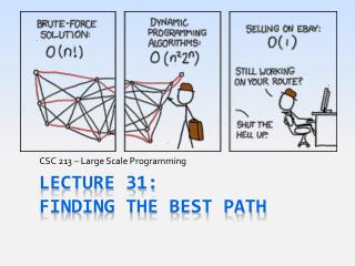
Graph Search Algorithms • Breadth-first Search • Depth-first Search • Bidirectional Search • Greedy Best-first Search • A* Search
Breadth-first Search(BFS) 以起點為中心,由近而遠地全面往「外」搜尋,直至碰到目標點為止。 優點:保證可找到最短路徑。 缺點:需要用大量的記憶體來儲存已展開但尚未檢視的節點。
Depth-first Search(DFS) 從起點開始,單線地往「前」搜尋。若無法再前進,則後退換另一條路線前進。搜尋直至碰到目標點為止。 優點:記憶體的需求較 BFS 低。 缺點:1. 若圖具有無限多個節點,可能無法走到目標。2. 找到的路徑也許不是最短的,
Bidirectional Search 從起點與終點用同樣的方法搜尋,直到發現交會點為止。找到的兩條路徑合併起來即為起點到終點的路徑。 優點:記憶體的需求較低。 缺點:程式比較複雜。
前述的 BFS 和 DFS 方法完全以圖的結構(即端點間的連接關係)來選擇下一個拜訪點。 另有一類搜尋演算法運用外在的資訊來選擇「可能更好」的下一個拜訪點,期望能更快地發現到達目標的路徑。這一類的演算法把已知和外在資訊轉化成一個函式 f(n)來計算端點 n目前的預估成本(estimated cost)。如果演算法永遠把具有最小函式值的已知但尚未拜訪的端點選擇為下一個拜訪點,則稱為 Best-first Search。 我們將用下一頁的 Romania 簡化地圖為例來介紹兩種 Best-first Search: Greedy Best-first Search 和 A* Search。
start goal 簡化的 Romania 地圖
Greedy Best-first Search • heuristic function h(n) 的定義如下: • h(n) = 從端點 n到目標點路徑的最低成本預估值 • 此演算法把 h(n) 選為前述的 f(n),即 f(n) = h(n)。 • 以 Romania 地圖為例來說,我們可以定義 • h(n) = hSLD(n) = 都市 n和目標都市 Bucharest 的直線距離 • 下一頁表列出 hSLD(n) 的值。
start goal solution 前述演算法實作時必須考慮 backtracking 與排除迴路情況(如 Iasi 與 Neamt 之間)
A* Search • A*(讀作 A-star)是最著名的 best-first 搜尋法。它的函式 f(n) 定義如下: • f(n) = g(n) + h(n) • 其中,h(n) 如前所述,g(n) 則是從起點到端點 n路徑的真實成本。因此, • f(n) = 經過端點 n 所有路徑的最低預估成本 • 譬如:下兩頁顯示 A* 搜尋 Romania 地圖的過程。
start goal
A* Tree Search Algorithm • function Search (start, goal) • pool← {start}; • loop do • if pool is empty return failure; • node← 從 pool集合中取出 f值最小的端點; • if node is goal then return the solution path; • 把與 node相鄰的端點加入集合 pool中; ※ 端點可重複展開 註:1. 集合 pool可以用資料結構 priority queue 來製作。 2. 可以在 node中記錄 parent 端點,藉以反求出 起點到終點的路徑。
A* Graph Search Algorithm • function Search (start, goal) • closed← empty set; // 存放已展開過的端點 • open← {start}; • loop do • if open is empty return failure; • node← 從 open中取出 f值最小的端點; • if node is goal then return the solution path; • if node不在集合 closed中 • 把 node加入集合 closed 中; • 把與 node相鄰的端點加入集合 open 中; ※ 端點不可重複展開
h(n) n goal c(n, a, n') h(n') n' • A heuristic h(n) is admissible if it never overestimates the cost to reach the goal. • A heuristic h(n) is consistent if, for every node n and every successor node n' of n generated by any action a, the following inequality holds: • h(n) c(n, a, n') + h(n') • where c(n, a, n') is the cost from n to n' due to action a.
假定 C*是最佳路徑的成本。 • f(G') = g(G') + h(G') = g(G') > C* • 若 n是最佳路徑上的一個節點,則 • f(n) = g(n) + h(n) C* • 所以 • f(n) C* < f(G') • 因此演算法會選擇節點 n展開,繼續尋找最佳路徑。 start optimal path = 0 n G' G 若 h(n) 是 admissible,則 A* Tree Search 演算法找出的路徑一定是最佳路徑。 不在最佳路徑上的目標點
若 h(n) 是 consistent,則 A* Graph Search 演算法找出的路徑一定是最佳路徑。 • 假定 m是 n在某路徑中的後繼節點。由 consistent 的定義,我們得到: • f(m) = g(m) + h(m) = g(n) + c(n, a, m) + h(m) g(n) + h(n) • 所以 f 沿著路徑, 是一個非遞減函式。 • 因此,當演算法碰到第一個可展開的目標節點時,即找到了最佳的路徑。
Map Search Structures • Retangular grid • Quadtree • Convex polygons • Points of visibility
goal start
References Books Andre LaMothe. Tricks of the Windows Game Programming Gurus. SAMS. 1999. S. Russell and P. Norvig. Artifucial Intelligence: A Modern Approach 2nd Ed. Prentice Hall. 2003. Mark DeLoura. Game Programming Gems. Charles River Media, Inc. 2000 Websites: Amit's Thoughts on Path-Finding and A-Star (http://theory.stanford.edu/~amitp/GameProgramming/)


![AI pada Game Development [Path Finding]](https://cdn1.slideserve.com/3600279/ai-pada-game-development-path-finding-dt.jpg)