Download
1 / 49
490 likes | 633 Views
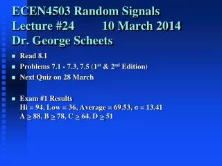
ECEN4503 Random Signals Lecture #27 11 March 2013 Dr. George Scheets. Read 8.5 Problems: 5.22, 8.3, 8.5, 8.6 (1st Edition) Problems: 5.51, 8.8, 8.9, 8.10 (2nd Edition). ECEN4503 Random Signals Lecture #29 15 March 2013 Dr. George Scheets.

E N D
ECEN4503 Random SignalsLecture #27 11 March 2013Dr. George Scheets • Read 8.5 • Problems: 5.22, 8.3, 8.5, 8.6(1st Edition) • Problems: 5.51, 8.8, 8.9, 8.10 (2nd Edition)
ECEN4503 Random SignalsLecture #29 15 March 2013Dr. George Scheets • Problems 8.7a & b, 8.11, 8.12a-c (1st Edition) • Problems 8.11a & b, 8.15, 8.16 (2nd Edition)
Random Process X(t) Set of possible time domain waveforms Associated with some experiment x(t) = a specific waveform from X(t) Freeze Time at, say, t1X(t1) = set of points = X (Random Variable) one point from each waveform taken at same time (t1) Set of points has... Histogram → PDF, E[X], σ2X, etc.
Random Process Stat Averages taken ┴ to time axis Using a point from every single waveformNot practical in Real World Time Averages taken along time axis Using one waveform x(t) Time Averages = Statistical Averages?Process is said to be Ergodic. Cautiously treat all processes in this class as ergodic.
Some Waveforms Aren't Ergodic • Random DC voltage • x(t) might be, say, +2.3556 volts DC • X(t) might be the set of all DC waveformsfrom, say, -5 vdc to +5 vdc • E[X(t)] would = 0 vdc • If waveforms equally likely • A[x(t)] would = 2.3556 vdc
Ergodic Process X(t) volts • E[X] = A[x(t)] volts • Mean • Average • Average Value • Vdc on multi-meter • E[X]2 = A[x(t)]2volts2 • (Normalized) D.C. power watts
Ergodic Process • E[X2] = A[x(t)2] volts2 • 2nd Moment • (Normalized) Average Power watts • (Normalized) Total Power watts • (Normalized) Average Total Power watts • (Normalized) Total Average Power watts
Ergodic Process • E[X2] - E[X]2 volts2 • A[x(t)2] - A[x(t)]2 • Variance σ2X • (Normalized) AC Power watts • E[(X -E[X])2] = A[(x(t) -A[x(t)])2] • Standard Deviation σXAC Vrms on multi-meter volts
PDF of a 3vp Sinusoid Area under PDF E[X2] Find PDF of voltage by treating Time as Uniform RV. Then map time → voltage. A[*] = E[*] when Ergodic.
Voltage PDF for Clean Sinusoid If x(t) = α cos(2πβt + θ)thenfX(x) = 1 / [π(α2 - x2)0.5]; - α < x <α
Given some waveform x(t)... • To find voltage PDF • Randomly sample waveformVisualize resulting Histogram • Mapping from 1 R.V. to AnotherMap time (t) → voltage (x)Treat time as Uniformly Distributed R.V.Treat waveform x(t) as mapping g(t) x (voltage) = g(t)
Stationary Process • Statistics (such as Mean, Variance, PDF, etc.) collected at different times are ≈ the same. • There are actually several "sub definitions" of stationarity, but we'll only worry about this one.
1.25 1 x i 0 1 1 0 20 40 60 80 100 0 i 100 100 bps Continuous Random Bit Stream with S.I. bits. P(+1 volt) = P(-1 volt) = 0.5 Several hundred bits collected at different times? Stationary Process. Voltage statistics should be similar. Several hundred samples collected over a nsec? Not stationary. Statistics may differ.
Internet Packet Traffic (Daily) Amsterdam Internet Exchange Internet traffic rate logged several thousand times over one hour periods? Not a stationary process. A process somewhat periodic is called cyclo-stationary.
Internet Packet Traffic (Annual) Amsterdam Internet Exchange Internet traffic rate logged several thousand times over monthly periods? Not a stationary process. Mean is increasing. Looks like variance is increasing too (swings get wider).
Annual Rainfall in SW USA Source: November 2007 National Geographic Daily rainfall amounts noted over a one year period? Not Stationary. This is probably a stationary process if the inputs to this experiment, sun output and environment factors, are constant.
MELP Voice Coder • NATO Standard • Developed Using American Voices • Quality degrades a bit in other languages • Phoneme statistics aren't the same • Smallest contrastive unit of sound
Review of PDF's & Histograms Probability Density Functions (PDF's), of which a Histogram is an estimate of shape, frequently (but not always!) deal with the voltage likelihoods Volts Time
Discrete Time Noise Waveform255 point, 0 mean, 1 wattUniformly Distributed Voltages Volts 0 Time
15 Bin Histogram(255 points of Uniform Noise) Bin Count 0 Volts
15 Bin Histogram(2500 points of Uniform Noise) Bin Count When bin count range is from zero to max value, a histogram of a uniform PDF source will tend to look flatter as the number of sample points increases. 200 0 0 Volts
15 Bin Histogram(2500 points of Uniform Noise) Bin Count But there will still be variation if you zoom in. 200 140 0 Volts
15 Bin Histogram(25,000 points of Uniform Noise) 2,000 Bin Count 0 0 Volts
Bin Count Volts Time Volts The histogram is telling us which voltages were most likely in this experiment. A histogram is an estimate of the shape of the underlying PDF. 0
Discrete Time Noise Waveform255 point, 0 mean, 1 wattExponentially Distributed Voltages Volts 0 Time
15 bin Histogram(255 points of Exponential Noise) Bin Count 0 Volts
Discrete Time Noise Waveform255 point, 0 mean, 1 wattGaussian Distributed Voltages Volts 0 Time
15 bin Histogram(255 points of Gaussian Noise) Bin Count 0 Volts
15 bin Histogram(2500 points of Gaussian Noise) Bin Count 400 0 Volts
Autocorrelation Statistical average E[X(t)X(t+τ)] using Random Processes & PDF's Time average A[x(t)x(t+τ)] using a single waveform How alike is a waveform & shifted version of itself? Given an arbitrary point on the waveform x(t1), how predictable is a point τ seconds away at x(t1+τ)? RX(τ) = 0? Not alike. Uncorrelated. RX(τ) > 0? Alike. Positively correlated. RX(τ) < 0? Opposite. Negatively correlated.
Time Average vs Statistical Average t1 + T ∞ A[ ? ] = lim (1/T) ? dt T →∞ t1 -∞ E[ ? ] = ? fX(x) dx
Need to find the Autocorrelation? t1 + T = t2 • Take the time average!!! t1 RXX(τ) = lim (1/T) x(t)x(t+τ) dt T →∞
Volts Time PDF's & Histograms • Voltage Probability Density Functions (PDF's), of which a Histograms is an estimate of shape, deal with the voltage likelihoods
1.25 1.25 1 1 x x i i 0 0 1 1 1 1 0 50 100 150 200 250 300 350 400 0 20 40 60 80 100 0 i 400 0 i 100 These waveforms have same Voltage PDF's
Volts time Review of Autocorrelation • Autocorrelations deal with predictability over time. I.E. given an arbitrary point x(t1), how predictable is x(t1+τ)? τ t1
Review of Autocorrelation t1 + T = t2 Rx(τ) = lim (1/T) x(t)x(t+τ) dt T →∞ Take x(t1)*x(t1+ τ), x(t1+ε)*x(t1+ τ + ε)... ....x(t2)*x(t2+ τ)... Add these all together, then average. t1
Review of Autocorrelation N-τ ∑ Rx(τ) = 1/(N-τ) x(i)x(i+τ) i=1 Example: Rx(0) for discrete time signal ... ... x(i+0) x(1) x(2) x(3) x(100) x(i) x(1) x(2) x(3) x(100) Sum up x(1)2 + x(2)2 + ... + x(100)2, Then take a 100 point average.
Review of Autocorrelation Example: Rx(1) for discrete time signal x(t+1) x(1) x(2) x(3) x(100) x(t) x(1) x(2) x(3) x(99) x(100) Sum up x(1)x(2) + x(2)x(3) + ... + x(99)x(100), Then average. If average is negative, paired numbers must tend to have opposite sign.
Review of Autocorrelation Example: Rx(2) for discrete time signal x(t+2) x(1) x(2) x(3) x(100) x(t) x(1) x(2) x(98) x(99) Sum up x(1)x(3) + x(2)x(4) + ... + x(98)x(100), Then average. If average is near zero, paired numbers must tend to have unpredictable signs.
255 point discrete time Exponentially Distributed Noise Waveform(Adjacent points are independent) Vdc = 0 v, Normalized Power = 1 watt Volts 0 time
255 point discrete time Gaussian Distributed Noise Waveform(Adjacent points are independent) Vdc = 0 v, Normalized Power = 1 watt Volts 0 time
255 point discrete time Uniformly Distributed Noise Waveform(Adjacent points are independent) Vdc = 0 v, Normalized Power = 1 watt Volts 0 time
Autocorrelation Estimate of Discrete Time White Noise Rxx The previous 3 waveforms all have the same theoretical autocorrelation function. 1 0 tau (samples)
255 point Noise Waveform(Low Pass Filtered White Noise) 23 points Volts 0 Time
Autocorrelation Estimate of Low Pass Filtered White Noise Rxx 0 23 tau samples
1.25 1 x i 0 1 1 0 20 40 60 80 100 0 i 100 40 32 20 rx j 0 3 20 0 10 20 30 40 50 60 0 j 60 Autocorrelation of Random Bit StreamEach bit randomly Logic 1 or 0 1
1.25 1 x i 0 40 32 20 1 1 0 50 100 150 200 250 300 350 400 rx j 0 i 400 0 6 20 0 10 20 30 40 50 60 0 j 60 Bit Stream #2Logic 1 & 0 bursts of 20 bits (on average) 1