Decision Trees
Learn about decision tree induction, including ID3, C4.5, and CART algorithms, attribute selection methods, information gain calculations, and the computational complexity involved. Understand how decision trees are built and the process of splitting criteria.


Decision Trees
E N D
Presentation Transcript
Decision tree induction is the learning of decision trees from class-labelled training examples. • A decision-tree is a flow-chart like tree structure, where each internal node denotes a test on an attribute, each branch represents an outcome of the test and each leaf node holds a class label.
Decision Tree Induction • ID3 Iterative Dichotomiser 3 by J. Ross Quinlan • C4.5 is a successor of ID3 • Classification and Regression Trees(CART) – generation of binary trees
ID3, C4.5 and CART adopt a greedy(nonbacktracking) approach in which decision trees are constructed in a top-down recursive divide-and-conquer manner. • Algorithm starts with a training set of tuples and their associated class labels. • Training stet is recursively partitioned into smaller subsets as the tree is being built.
The Algorithm • Create a root node N for the tree • If all examples are of same class C, then return N as the leaf node labeled with the class C. • If attribute_list is empty, then return N as the leaf node labeled with the majority class in D(majority voting)
Apply Attribute_Selection_method(D, attribute_list) to find “best” splitting_criteria; • Label node N with splitting_criterion • If splitting_attribute is discrete_valued and multiway splits allowed then • attribute_list attribute_list – splitting_attribute
For each outcome j of splitting_criterion Let Dj be the set of data tuples in D satisfying outcome j; If Dj is empty then • Attach a leaf labelled with the majority class in D to node N; else • Attach the node returned by Generate_decision_tree(Dj, attribute_list) to node N • Endfor • Return N
To partition attributes in D, there are three possible scenarios. Let A be the splitting attribute. A has v distinct values, {a1,a2,…,av}, based on training data. • A is discrete-valued: • A is continuous-valued: • A is discrete-valued and a binary tree must be produced.
The recursive partitioning stops only when one of the following terminating condition is true: • All the tuples in partition D belong to the same class • There are no remaining attributes on which the tuples may be further partitioned. In this case majority voting is employed. • There are no tuples for a given branch, that is, a partition Dj, is empty. In this case, a leaf is created with the majority class in D. • What is the computational complexity?
Attribute Selection Procedure • It is a heuristic for selecting the splitting criterion that “best” separates a given data partition, D, of class-labelled training tuples into individual classes. • It is also known as splitting rules because they determine how the tuples at a given node are to be split. • It provides ranking for each attribute describing the given training tuple. The attribute having the best score for the measure is chosen as the splitting attribute for the given tuples. • Well known attribute selection measures are : information gain, gain ratio, gini index.
Information Gain(ID3/C4.5) • Select the attribute with the highest information gain. • Let pi be the probability that an arbitrary tuple in D belongs to class Ci, estimated by |Ci, D|/|D| • Expected information (entropy) needed to classify a tuple in D:
Information needed (after using A to split D into v partitions) to classify D: • Information gained by branching on attribute A
Exercise • Calculate the information(entropy) • Given: • Set S contains14 examples • 9 Positive values • 5 Negative values
Exercise • Info(S) = - (9/14) log2 (9/14) - (5/14) log2 (5/14) • = 0.940
Information Gain • Information gain is based on the decrease in entropy after a dataset is split on an attribute. • Looking for which attribute creates the most homogeneous branches
Information Gain Example • 14 examples, 9 positive 5 negative • The attribute is Wind. • Values of wind are Weak and Strong
Exercise (cont.) • 8 occurrences of weak winds • 6 occurrences of strong winds • For the weak winds, 6 are positive and 2 are negative • For the strong winds, 3 are positive and 3 are negative
Exercise (cont.) • Gain(S,Wind) = • Info(S) - (8/14) * Info(Weak) -(6/14) * Info(Strong) • Info(Weak) = - (6/8)*log2(6/8) - (2/8)*log2(2/8) = 0.811 • Info(Strong) = - (3/6)*log2(3/6) - (3/6)*log2(3/6) = 1.00
Exercise (cont.) • So… • 0.940 - (8/14)*0.811 - (6/14)*1.00 • = 0.048
Sample training data to determine whether an animal lays eggs.
Entropy(4Y,2N): -(4/6)log2(4/6) – (2/6)log2(2/6) = 0.91829 Now, we have to find the IG for all four attributes Warm-blooded, Feathers, Fur, Swims
For attribute ‘Warm-blooded’: Values(Warm-blooded) : [Yes,No] S = [4Y,2N] SYes = [3Y,2N] E(SYes) = 0.97095 SNo = [1Y,0N] E(SNo) = 0 (all members belong to same class) Gain(S,Warm-blooded) = 0.91829 – [(5/6)*0.97095 + (1/6)*0] = 0.10916 For attribute ‘Feathers’: Values(Feathers) : [Yes,No] S = [4Y,2N] SYes = [3Y,0N] E(SYes) = 0 SNo = [1Y,2N] E(SNo) = 0.91829 Gain(S,Feathers) = 0.91829 – [(3/6)*0 + (3/6)*0.91829] = 0.45914
For attribute ‘Fur’: Values(Fur) : [Yes,No] S = [4Y,2N] SYes = [0Y,1N] E(SYes) = 0 SNo = [4Y,1N] E(SNo) = 0.7219 Gain(S,Fur) = 0.91829 – [(1/6)*0 + (5/6)*0.7219] = 0.3167 For attribute ‘Swims’: Values(Swims) : [Yes,No] S = [4Y,2N] SYes = [1Y,1N] E(SYes) = 1 (equal members in both classes) SNo = [3Y,1N] E(SNo) = 0.81127 Gain(S,Swims) = 0.91829 – [(2/6)*1 + (4/6)*0.81127] = 0.04411
Gain(S,Warm-blooded) = 0.10916 Gain(S,Feathers) = 0.45914 Gain(S,Fur) = 0.31670 Gain(S,Swims) = 0.04411 Gain(S,Feathers) is maximum, so it is considered as the root node Feathers Y N [Ostrich, Raven, Albatross] [Crocodile, Dolphin, Koala] Lays Eggs ? The ‘Y’ descendant has only positive examples and becomes the leaf node with classification ‘Lays Eggs’
We now repeat the procedure, S: [Crocodile, Dolphin, Koala] S: [1+,2-] Entropy(S) = -(1/3)log2(1/3) – (2/3)log2(2/3) = 0.91829
For attribute ‘Warm-blooded’: Values(Warm-blooded) : [Yes,No] S = [1Y,2N] SYes = [0Y,2N] E(SYes) = 0 SNo = [1Y,0N] E(SNo) = 0 Gain(S,Warm-blooded) = 0.91829 – [(2/3)*0 + (1/3)*0] = 0.91829 For attribute ‘Fur’: Values(Fur) : [Yes,No] S = [1Y,2N] SYes = [0Y,1N] E(SYes) = 0 SNo = [1Y,1N] E(SNo) = 1 Gain(S,Fur) = 0.91829 – [(1/3)*0 + (2/3)*1] = 0.25162 For attribute ‘Swims’: Values(Swims) : [Yes,No] S = [1Y,2N] SYes = [1Y,1N] E(SYes) = 1 SNo = [0Y,1N] E(SNo) = 0 Gain(S,Swims) = 0.91829 – [(2/3)*1 + (1/3)*0] = 0.25162 Gain(S,Warm-blooded) is maximum
The final decision tree will be: Feathers Y N Lays eggs Warm-blooded Y N Does not lay eggs Lays Eggs
S = [3+, 5-] Entropy(S) = -(3/8)log2(3/8) – (5/8)log2(5/8) = 0.95443 Find IG for all 4 attributes: Hair, Height, Weight, Lotion For attribute ‘Hair’: Values(Hair) : [Blonde, Brown, Red] S = [3+,5-] SBlonde = [2+,2-] E(SBlonde) = 1 SBrown = [0+,3-] E(SBrown) = 0 SRed = [1+,0-] E(SRed) = 0 Gain(S,Hair) = 0.95443 – [(4/8)*1 + (3/8)*0 + (1/8)*0] = 0.45443
For attribute ‘Height’: Values(Height) : [Average, Tall, Short] SAverage = [2+,1-] E(SAverage) = 0.91829 STall = [0+,2-] E(STall) = 0 SShort = [1+,2-] E(SShort) = 0.91829 Gain(S,Height) = 0.95443 – [(3/8)*0.91829 + (2/8)*0 + (3/8)*0.91829] = 0.26571 For attribute ‘Weight’: Values(Weight) : [Light, Average, Heavy] SLight = [1+,1-] E(SLight) = 1 SAverage = [1+,2-] E(SAverage) = 0.91829 SHeavy = [1+,2-] E(SHeavy) = 0.91829 Gain(S,Weight) = 0.95443 – [(2/8)*1 + (3/8)*0.91829 + (3/8)*0.91829] = 0.01571 For attribute ‘Lotion’: Values(Lotion) : [Yes, No] SYes = [0+,3-] E(SYes) = 0 SNo = [3+,2-] E(SNo) = 0.97095 Gain(S,Lotion) = 0.95443 – [(3/8)*0 + (5/8)*0.97095] = 0.01571
Gain(S,Hair) = 0.45443 Gain(S,Height) = 0.26571 Gain(S,Weight) = 0.01571 Gain(S,Lotion) = 0.3475 Gain(S,Hair) is maximum, so it is considered as the root node Hair Blonde Brown Red [Sarah, Dana, Annie, Katie] [Alex, Pete, John] Not Sunburned ? [Emily] Sunburned
Repeating again: S = [Sarah, Dana, Annie, Katie] S: [2+,2-] Entropy(S) = 1 Find IG for remaining 3 attributes Height, Weight, Lotion • For attribute ‘Height’: Values(Height) : [Average, Tall, Short] S = [2+,2-] SAverage = [1+,0-] E(SAverage) = 0 STall = [0+,1-] E(STall) = 0 SShort = [1+,1-] E(SShort) = 1 Gain(S,Height) = 1 – [(1/4)*0 + (1/4)*0 + (2/4)*1] = 0.5
For attribute ‘Weight’: Values(Weight) : [Average, Light] S = [2+,2-] SAverage = [1+,1-] E(SAverage) = 1 SLight = [1+,1-] E(SLight) = 1 Gain(S,Weight) = 1 – [(2/4)*1 + (2/4)*1]= 0 For attribute ‘Lotion’: Values(Lotion) : [Yes, No] S = [2+,2-] SYes = [0+,2-] E(SYes) = 0 SNo = [2+,0-] E(SNo) = 0 Gain(S,Lotion) = 1 – [(2/4)*0 + (2/4)*0]= 1 Therefore, Gain(S,Lotion) is maximum
In this case, the final decision tree will be Hair Blonde Brown Red Sunburned Not Sunburned Lotion N Y Not Sunburned Sunburned
Computing Information-Gain for Continuous-Valued Attributes • Let attribute A be a continuous-valued attribute • Must determine the best split point for A • Sort the value A in increasing order • Typically, the midpoint between each pair of adjacent values is considered as a possible split point • (ai+ai+1)/2 is the midpoint between the values of ai and ai+1 • The point with the minimum expected information requirement for A is selected as the split-point for A • Split: • D1 is the set of tuples in D satisfying A ≤ split-point, and D2 is the set of tuples in D satisfying A > split-point
Gain Ratio for Attribute Selection (C4.5) • Information gain measure is biased towards attributes with a large number of values • C4.5 (a successor of ID3) uses gain ratio to overcome the problem (normalization to information gain) • GainRatio(A) = Gain(A)/SplitInfo(A) • Ex. • gain_ratio(income) = 0.029/1.557 = 0.019 • The attribute with the maximum gain ratio is selected as the splitting attribute
Gini Index (CART, IBM IntelligentMiner) • If a data set D contains examples from n classes, gini index, gini(D) is defined as where pj is the relative frequency of class j in D • If a data set D is split on A into two subsets D1 and D2, the gini index gini(D) is defined as • Reduction in Impurity: • The attribute provides the smallest ginisplit(D) (or the largest reduction in impurity) is chosen to split the node (need to enumerate all the possible splitting points for each attribute)
Computation of Gini Index • Ex. D has 9 tuples in buys_computer = “yes” and 5 in “no” • Suppose the attribute income partitions D into 10 in D1: {low, medium} and 4 in D2 Gini{low,high} is 0.458; Gini{medium,high} is 0.450. Thus, split on the {low,medium} (and {high}) since it has the lowest Gini index • All attributes are assumed continuous-valued • May need other tools, e.g., clustering, to get the possible split values • Can be modified for categorical attributes
Comparing Attribute Selection Measures • The three measures, in general, return good results but • Information gain: • biased towards multivalued attributes • Gain ratio: • tends to prefer unbalanced splits in which one partition is much smaller than the others • Gini index: • biased to multivalued attributes • has difficulty when # of classes is large • tends to favor tests that result in equal-sized partitions and purity in both partitions
Other Attribute Selection Measures • CHAID: a popular decision tree algorithm, measure based on χ2 test for independence • C-SEP: performs better than info. gain and gini index in certain cases • G-statistic: has a close approximation to χ2 distribution • MDL (Minimal Description Length) principle (i.e., the simplest solution is preferred): • The best tree as the one that requires the fewest # of bits to both (1) encode the tree, and (2) encode the exceptions to the tree • Multivariate splits (partition based on multiple variable combinations) • CART: finds multivariate splits based on a linear comb. of attrs. • Which attribute selection measure is the best? • Most give good results, none is significantly superior than others
Preparing Data for Classification and Prediction • Data Cleaning : remove or reduce noise (apply smoothing) and treatment of missing values (replacing a missing value with the most commonly occurring values for that attribute, or with the most probable value based on statistics) • Relevance Analysis : 1) Correlation analysis is used to check whether any two given attributes are statistically related. 2) Dataset may also contain irrelevant attributes. These kind of attributes may otherwise slow down and possibly mislead the learning step. • Data Transformation and Reduction : may be transformed by normalization – scaling attributes such that it comes in one range. Or by generalizing it to higher-level concepts.
Advantage of ID3 • Understandable prediction rules are created from the training data. • Builds the fastest tree. • Builds a short tree. • Only need to test enough attributes until all data is classified. • Finding leaf nodes enables test data to be pruned, reducing number of tests.
Disadvantage of ID3 • Data may be over-fitted or over-classified, if a small sample is tested. • Only one attribute at a time is tested for making a decision. • Classifying continuous data may be computationally expensive, as many trees must be generated to see where to break the continuum.
Bayes’ Theorem: Basics • Total probability Theorem: • Bayes’ Theorem: • Let X be a data sample (“evidence”): class label is unknown • Let H be a hypothesis that X belongs to class C • Classification is to determine P(H|X), (i.e., posteriori probability): the probability that the hypothesis holds given the observed data sample X • P(H) (prior probability): the initial probability • E.g., X will buy computer, regardless of age, income, … • P(X): probability that sample data is observed • P(X|H) (likelihood): the probability of observing the sample X, given that the hypothesis holds • E.g.,Given that X will buy computer, the prob. that X is 31..40, medium income
Prediction Based on Bayes’ Theorem • Given training dataX, posteriori probability of a hypothesis H, P(H|X), follows the Bayes’ theorem • Informally, this can be viewed as posteriori = likelihood x prior/evidence • Predicts X belongs to Ci iff the probability P(Ci|X) is the highest among all the P(Ck|X) for all the k classes • Practical difficulty: It requires initial knowledge of many probabilities, involving significant computational cost