Active Set Support Vector Regression
Active Set Support Vector Regression. David R. Musicant Alexander Feinberg NIPS 2001 Workshop on New Directions in Kernel-Based Learning Methods Friday, December 7, 2001. Carleton College. Active Set Support Vector Regression. Fast algorithm that utilizes an active set method

Active Set Support Vector Regression
E N D
Presentation Transcript
Active SetSupport Vector Regression David R. Musicant Alexander Feinberg NIPS 2001 Workshop on New Directions in Kernel-Based Learning Methods Friday, December 7, 2001 Carleton College
Active Set Support Vector Regression • Fast algorithm that utilizes an active set method • Requires no specialized solvers or software tools, apart from a freely available equation solver • Inverts a matrix of the order of the number of features (in the linear case) • Guaranteed to converge in a finite number of iterations
The Regression Problem • “Close points” may be wrong due to noise only • Line should be influenced by “real” data, not noise • Ignore errors from those points which are close!
Measuring Regression Error • Given m points in the n dimensional space Rn • Represented by an mx n matrix A • Associated with each point Ai is an observation yi • Consider a plane to fit the data, and a “tube” of width e around the data. Measure error outside the tube: • where e is a vector of ones.
Support Vector Regression • Traditional support vector regression: • Minimize the error made outside of the tube • Regularize the fitted plane by minimizing the norm of w • The parameter C balances two competing goals
Our reformulation • Allow regression error ( ) to contribute in a quadratic fashion, instead of linearly. • Regularize regression plane with respect to location (b) in addition to orientation (w). • Non-negativity constraints for slack variables are no longer necessary. plane “orientation” regression error plane “location”
Wolfe Dual Formulation • The dual formulation can be represented as: where • Non-negativity constraints only • = dual variables • Nasty objective function
Simpler Dual Formulation • At optimality, . • Add this as a constraint, and simplify objective: • I = identity matrix • Complementarity condition introduced to simplify objective function • The only constraints are non-negativity and complementarity
Active Set Algorithm: Idea • Partition dual variables into nonbasic variables: basic variables: • Algorithm is an iterative method. • Choose a working set of variables corresponding to active constraints to be nonbasic • Choose variables so as to preserve complementarity • Calculate the global minimum on basic variables • Appropriately update working set • Goal is to find appropriate working set. • When found, global minimum on basic variables is solution to problem
Active Set Algorithm: Basics • Definition: • At each iteration, redefine basic and nonbasic sets: • Define: • Define:
Active Set Algorithm: Basics • Optimization problem, on an active set, becomes: • Complementarity constraint is implicit by choice of basic and nonbasic sets. • Find global minimum on basic set, then project.
Active Set Algorithm: Basics • Converting back from u: • When computing M-1, we use Sherman-Morrison-Woodbury identity: • To restate: • Like ASVM, the ASVR basic approach finds the minimum on a set of basic variables, then projects onto the feasible region. • This differs from other active set methods, which “backtrack” onto the feasible region.
Graphical Comparison Basic ASVR Step Standard Active Set Approach Feasible Region Feasible Region Initial point Initial point Projection Projection Minimum Minimum
Some additional details • When the basic ASVR step fails to make progress, we fall back on the standard active set approach. • When we no longer make any progress on the active set, we free all variables and use a gradient projection step. • Note: This step may violate complementarity! • Complementarity can be immediately restored with a shift.
Preserving Complementarity • Suppose there exists i such that • Defineand redefine • Then all terms of objective function above remain fixed, apart from last term which is reduced further. • Shift preserves complementarity and improves objective.
Experiments • Compared ASVR and its formulation with standard formulation via SVMTorch and mySVM • measured generalization error and running time • mySVM experiments only completed on smallest dataset, as it ran much more slowly than SVMTorch • Used tuning methods to find appropriate values for C • Synthetic dataset generated for largest test • All experiments run on: • 700 MHz Pentium III Xeon, 2 Gigabytes available memory • Red Hat Linux 6.2, egcs-2.91.66 C++ • Data was in core for these experiments. The algorithm can easily be extended for larger datasets. • Convergence is guaranteed in a finite number of iterations.
Experiments on Public Datasets • (*) indicates that we stopped tuning early due to long running times. The more we improved generalization error, the longer SVMTorch took to run. • ASVR has comparable test error to SVMTorch, and runs dramatically faster on the larger examples.
Experiment on Massive Dataset • SVMTorch did not terminate after several hours on this dataset, under a variety of parameter settings.
Conclusions • Conclusions: • ASVR is an active set method that requires no external optimization tools apart from a linear equation solver • Performs competitively with other well-known SVR tools (linear kernels) • Only a single matrix inversion in n+1 dimensions (where n is usually small) is required • Future work • Out-of-core implementation • Parallel processing of data • Kernel implementation • Integrating reduced SVM or other methods for reducing the number of columns in kernel matrix