Pulsar timing: how it works why it works how well can it work? Noise budget: Pulsar  Earth

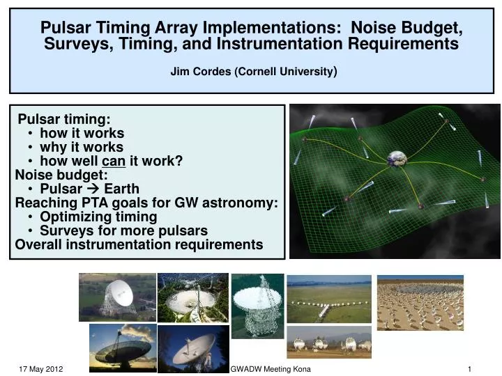
1. Pulsar Timing Array Implementations:  Noise Budget, Surveys, Timing, and Instrumentation Requirements Jim Cordes (Cornell University) • Pulsar timing: • how it works • why it works • how well can it work? • Noise budget: • Pulsar  Earth • Reaching PTA goals for GW astronomy: • Optimizing timing • Surveys for more pulsars • Overall instrumentation requirements GWADW Meeting Kona

2. Difficulties of GW Detection Pulsar Timing Array L ~ cT ~ 3 pc hmin ~ 10-16 – 10-14 ΔL ~ 103 to 105 cm Ground-based Interferometer L ~ 4 km hmin ~ 10-23 ΔL ~ 10-18 cm 10-3 RNS 10-5 Rnucleus • PTA: δt includes • Translational motion of the NS ~ 100 km/s • Orbital motions of the pulsar and observatory: 10s – 100s km/s • Interstellar propagation delays: ns to seconds GWADW Meeting Kona

3. The PTA Program • Goal • Detect GWs at levels h~10-15 at f~1 yr-1 • Stochastic backgrounds (e.g. SMBH binaries, strings) • Continuous waves • Bursts (including bursts with memory) • Broad requirements • Time 20 high-quality MSPs with < 100 ns rms precision over 5 to 10 yr for detection • Wideband receivers at 1 to 2 GHz • Confirmation and characterization of GWs: 50 MSPs • Understanding the noise budget • Galactic census for pulsars ~104 MSPs in the Milky Way (also NS-NS binaries, MSPs, NS-BH binaries, GC pulsars) GWADW Meeting Kona

4. Stochastic Background from SMBHs:Correlation Function Between Pulsars Example power-law spectrum from merging supermassive black holes (Jaffe & Backer 2003) Correlation function of residuals vs angle between pulsars Hellings-Downs angular correlation for Earth terms f-2/3 • Estimation errors from: • dipole term from solar system ephemeris errors • red noise in the pulsar clock • red interstellar noise GWADW Meeting Kona

5. Basics of Pulsars as Clocks MP • Signal average M pulses • Time-tag using template fitting … P W • Repeat for L epochs spanning N=T/P spin periods • N ~ 108 – 1010 cycles in one year •  P determined to • B1937+21: P = 0.00155780649243270.0000000000000004 s • J1909-3744:eccentricity < 0.00000013 (Jacoby et al.) GWADW Meeting Kona

6. Fundamentals of Pulsar Timing GWADW Meeting Kona

7. To pulsar Earth Roemer delay 500 s Solar system barycenter is near the sun’s photosphere Topocentric arrival times  solar system barycenter (SSBC) Pulse phase model is evaluated at the SSBC GWADW Meeting Kona

8. Simulated results for a millisecond pulsar Deterministic terms in the clock phase (t) Spin noise due to torque fluctuations (e.g. crust-core interactions) GWADW Meeting Kona

9. Using Pulsars as Clocks: Precision Timing of Pulsars Differential rotation, superfluid vortices Uncertainties in planetary ephemerides and propagation in interplanetary medium Interstellar dispersion and scattering Glitches Spin noise Magnetosphere Emission region: beaming and motion GPS time transfer Additive noise Instrumental polarization GWADW Meeting Kona

10. The clock is not perfect The spinning NS = the clock ~ 10 km radius Single pulses: phase jitter + amplitude modulations B0943+10 Rosen & Clemens 2008 Crab pulsar shot pulses (ns) Hankins & Eilek 2007 Relativistic emission regions magnetosphere ~ 100 – 104 km GWADW Meeting Kona

11. Why Millisecond Pulsars? Low intrinsic spin noise: Low magnetic fields (108-109 G)  long evolution times (> Gyr)  small torques Small pulse widths (10s – 100s μs)  more accurate time-tagging Small spin periods  many pulses per unit telescope time  Some TOA errors ~ 1 / (Number of pulses)1/2 Small magnetospheres (cP/2π)  inability for debris to enter and induce torque variations Millisecond pulsars with white-dwarf companions: dynamically clean GWADW Meeting Kona

12. GWADW Meeting Kona

13. 40 ΔTOA (µs) -50 0 18 Time (yr) B1937+21 SC10: scaling law for MSPs + CPs: α = -1.4; β = 1.1; γ = 2.0 For these pulsars, the residuals are mostly caused by spin noise in the pulsar: torque fluctuations crust quakes superfluid-crust interactions Other pulsars: excess residuals are caused by orbital motion (planets, WD, NS), ISM variations; Potentially: BH companions, gwaves, etc. GWADW Meeting Kona

14. Best timing residuals versus time:Demorest et al. 2012 J1713+0747 J1909-3744 GWADW Meeting Kona

15. Timing Error from Radiometer Noise rms TOA error from template fitting with additive noise: Interstellar pulse broadening, when large, increases ΔtS/N in two ways: • SNR decreases by a factor W / [W2+τd2]1/2 • W increases to [W2+τd2]1/2  Large errors for high DM pulsars and low-frequency observations Gaussian shaped pulse: Low-DM pulsars: DISS (and RISS) will modulate SNR N6 = N / 106 GWADW Meeting Kona

16. Timing Error from Pulse-Phase Jitter • fϕ = PDF of phase variation • a(ϕ) = individual pulse shape • Ni = number of independent pulses summed • mI = intensity modulation index ≈ 1 • fJ = fraction jitter parameter = ϕrms / W ≈ 1 Gaussian shaped pulse: N6 = Ni / 106 GWADW Meeting Kona

17. Propagation through the interstellar plasma birefringence GWADW Meeting Kona

18. Arecibo WAPP A Single Dispersed Pulse from the Crab Pulsar with coherent dedispersion S ~ 160 x Crab Nebula ~ 200 kJy Detectable to ~ 1.5 Mpc with Arecibo GWADW Meeting Kona

19. Interstellar Transfer Functions Dispersion: For narrow bandwidths and nonuniform ISM DM = dispersion measure Routinely measured to < 1 part in 104 GWADW Meeting Kona

20. Coherent Dedispersionpioneered by Tim Hankins (1971) Dispersion delays in the time domain represent a phase perturbation of the electric field in the Fourier domain: Coherent dedispersion involves multiplication of Fourier amplitudes by the inverse function, For the non-uniform ISM the deconvolution filter has just one parameter (DM) The algorithm consists of Application requires very fast sampling to achieve usable bandwidths. GWADW Meeting Kona

21. TOA Variations from electron density variations diffraction λ/ld Electron density irregularities from ~100s km to Galactic scales Trivial to correct if DM from mean electron density were the only effect! refraction GWADW Meeting Kona

22. Stochasticity of the PBF Speckles θy θx Nspeckles = Nscintles Nscintles = number of bright patches in the time-bandwdith plane Nscintles ≈ (1+η B/Δνd)(1+ηT/Δtd) GWADW Meeting Kona

23. Coherent Deconvolution of Scattering Broadening The impulse response for scattering gscattering(t) is of the form of envelope x noise process The noise process (from constructive/destructive interference) is constant over time scales ~100 s to hours. Algorithms being developed for extracting gscattering(t) to allow deconvolution and TOA correction GWADW Meeting Kona

24. Refraction in the ISM • Phase gradient in screen: • refraction of incident radiation • yields change in angle of arrival (AOA) • Two timing perturbations: • extra delay • error in correction to SSBC • Phase curvature in screen: • refractive intensity variation (RISS) • change in shape of ray bundle • change in pulse broadening, C1 GWADW Meeting Kona

25. Timing Budget (short list) GWADW Meeting Kona

26. Long-term Goal: Full Galactic Census All-sky surveys with existing radio telescopes, SKA precursors, and eventually the SKA can find a large fraction of pulsars SKA = Square Kilometer Array GWADW Meeting Kona

27. Summary • Timing precision for millisecond pulsars has been demonstrated to be sufficient eventual GW detection: • 30 ns rms over 5 yr for three objects • Work needed to characterize the noise budget (astrophysical and instrumental) for σTOA < 100 ns for a large sample of MSPs • A larger sample of MSPs ensures greater sensitivity by exploiting the correlated signal produced by GWs • A full Galactic census will provide the best MSPs • Long-term timing may require a dedicated timing telescope: antenna array vs. large single reflector? • E.g. 100-300 m equivalent in the southern hemisphere GWADW Meeting Kona