Download
1 / 17
170 likes | 186 Views
This lecture discusses the functions and components of router microarchitecture, such as the crossbar, buffer, and arbiter. It also explores different interconnection network topologies and their impact on power consumption. The lecture covers topics like buffer management, control logic, and routing algorithms.

E N D
Lecture 23: Interconnection Networks • Topics: Router microarchitecture, topologies
Router Functions • Crossbar, buffer, arbiter, VC state and allocation, • buffer management, ALUs, control logic, routing • The on-chip network can contribute 10-35% of total chip • power; network delays can add tens of cycles to cache • and memory access • Typical on-chip network power breakdown: • 30% link • 30% buffers • 30% crossbar
Router Pipeline • Four typical stages: • RC routing computation: the head flit indicates the VC that it belongs to, the VC state is updated, the headers are examined and the next output channel is computed (note: this is done for all the head flits arriving on various input channels) • VA virtual-channel allocation: the head flits compete for the available virtual channels on their computed output channels • SA switch allocation: a flit competes for access to its output physical channel • ST switch traversal: the flit is transmitted on the output channel A head flit goes through all four stages, the other flits do nothing in the first two stages (this is an in-order pipeline and flits can not jump ahead), a tail flit also de-allocates the VC
Router Pipeline • Four typical stages: • RC routing computation: compute the output channel • VA virtual-channel allocation: allocate VC for the head flit • SA switch allocation: compete for output physical channel • ST switch traversal: transfer data on output physical channel STALL Cycle 1 2 3 4 5 6 7 Head flit Body flit 1 Body flit 2 Tail flit RC VA SA ST RC VA SA SA ST -- -- SA ST -- -- -- SA ST -- -- SA ST -- -- -- SA ST -- -- SA ST -- -- -- SA ST
Speculative Pipelines • Perform VA, SA, and ST in • parallel (can cause collisions • and re-tries) • Typically, VA is the critical • path – can possibly perform • SA and ST sequentially • Perform VA and SA in parallel • Note that SA only requires knowledge • of the output physical channel, not the VC • If VA fails, the successfully allocated • channel goes un-utilized Cycle 1 2 3 4 5 6 7 Head flit Body flit 1 Body flit 2 Tail flit RC VA SA ST RC VA SA ST -- SA ST SA ST -- SA ST SA ST -- SA ST SA ST • Router pipeline latency is a greater bottleneck when there is little contention • When there is little contention, speculation will likely work well! • Single stage pipeline?
Current Trends • Growing interest in eliminating the area/power overheads • of router buffers; traffic levels are also relatively low, so • virtual-channel buffered routed networks may be overkill • Option 1: use a bus for short distances (16 cores) and use • a hierarchy of buses to travel long distances • Option 2: hot-potato or bufferless routing
Centralized Crossbar Switch P0 P1 P2 P3 P4 P5 P6 P7
Crossbar Properties • Assuming each node has one input and one output, a • crossbar can provide maximum bandwidth: N messages • can be sent as long as there are N unique sources and • N unique destinations • Maximum overhead: WN2 internal switches, where W is • data width and N is number of nodes • To reduce overhead, use smaller switches as building • blocks – trade off overhead for lower effective bandwidth
Switch with Omega Network 000 P0 000 001 P1 001 010 P2 010 011 P3 011 100 P4 100 101 P5 101 110 P6 110 111 P7 111
Omega Network Properties • The switch complexity is now O(N log N) • Contention increases: P0 P5 and P1 P7 cannot • happen concurrently (this was possible in a crossbar) • To deal with contention, can increase the number of • levels (redundant paths) – by mirroring the network, we • can route from P0 to P5 via N intermediate nodes, while • increasing complexity by a factor of 2
Tree Network • Complexity is O(N) • Can yield low latencies when communicating with neighbors • Can build a fat tree by having multiple incoming and outgoing links P0 P1 P2 P3 P4 P5 P6 P7
Bisection Bandwidth • Split N nodes into two groups of N/2 nodes such that the • bandwidth between these two groups is minimum: that is • the bisection bandwidth • Why is it relevant: if traffic is completely random, the • probability of a message going across the two halves is • ½ – if all nodes send a message, the bisection • bandwidth will have to be N/2 • The concept of bisection bandwidth confirms that the • tree network is not suited for random traffic patterns, but • for localized traffic patterns
Distributed Switches: Ring • Each node is connected to a 3x3 switch that routes • messages between the node and its two neighbors • Effectively a repeated bus: multiple messages in transit • Disadvantage: bisection bandwidth of 2 and N/2 hops on • average
Distributed Switch Options • Performance can be increased by throwing more hardware • at the problem: fully-connected switches: every switch is • connected to every other switch: N2wiring complexity, • N2/4 bisection bandwidth • Most commercial designs adopt a point between the two • extremes (ring and fully-connected): • Grid: each node connects with its N, E, W, S neighbors • Torus: connections wrap around • Hypercube: links between nodes whose binary names differ in a single bit
Topology Examples Hypercube Grid Torus
k-ary d-Cube • Consider a k-ary d-cube: a d-dimension array with k • elements in each dimension, there are links between • elements that differ in one dimension by 1 (mod k) • Number of nodes N = kd (with no wraparound) Number of switches : Switch degree : Number of links : Pins per node : N Avg. routing distance: Diameter : Bisection bandwidth : Switch complexity : d(k-1)/2 2d + 1 d(k-1) Nd 2wkd-1 2wd (2d + 1)2 Should we minimize or maximize dimension?
Title • Bullet