Download
1 / 31
310 likes | 328 Views
Explore quantum dynamics and control of spins in diamond, discussing applications, spin manipulation, spin dynamics modeling, and combating decoherence. Learn about dynamical decoupling methods, novel protocols, and the role of advanced quantum control in nanoscale magnetic sensing and quantum technologies.

E N D
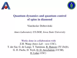
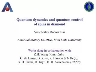
Quantum dynamics and quantum control of spins in diamond Viatcheslav Dobrovitski Ames Laboratory US DOE, Iowa State University Works done in collaboration with Z.H. Wang (Ames Lab), G. de Lange, D. Riste, R. Hanson (TU Delft), G. D. Fuchs, D. Toyli, D. D. Awschalom (UCSB)
Quantum spins in the solid state settings Quantum dots Magnetic molecules NV center in diamond Fundamental questions Applications How to manipulate quantum spins How to model spin dynamics Which dynamics is typical Which dynamics is interesting Which dynamics is useful Nanoscale magnetic sensing High-precision magnetometry Quantum repeaters Quantum key distribution Quantum memory
General problem: decoherence Decoherence: nuclear spins, phonons, conduction electrons, … Quantum control of spin state in presence of decoherence
Spin control – important topic (>10,000 items on Amazon.com)
Preserving coherence: dynamical decoupling (DD) Employ time reversal, like in spin echo Electron spin S Decohered by many nuclear spins Ik Spin echo: as if nothing happened Periodic DD (PDD): τ τ τ τ Central spin S is decoupled from the bath of spins Ik
Dynamical decoupling protocols General approach – e.g., group-theoretic methods Viola, Knill, Lloyd, PRL 1999 Examples: Periodic DD (CPMG, pulses along X): Period d-X-d-X (d – free evolution) Universal DD (2-axis, e.g. X and Y): Period d-X-d-Y-d-X-d-Y Can also choose XZ PDD, or YZ PDD – ideally, all the same (in reality, different)
Performance of DD and advanced protocols Assessing DD performance: Magnus expansion (asymptotic expansion for small delay τ, total experiment duration T ) Symmetrized XY PDD (XY SDD): XYXY-YXYX 2nd order protocol, error O(τ2) Concatenated XY PDD (CDD) level l=1 (CDD1 = PDD): d-X-d-Y-d-X-d-Y level l=2 (CDD2): PDD-X-PDD-Y-PDD-X-PDD-Y etc. Khodjasteh, Lidar, PRL 2005
Why we need something else? • Traditional NMR and ESR: • Only one spin component is preserved – others are often lost • Only macroscopic systems • Our focus: preserve complete quantum spin state for a single spin • Deficiencies of Magnus expansion: • Norm of H(0), H(1),… – grows with the size of the bath • Validity conditions are often not satisfied in reality • (but DD works) • Behavior at long times – unclear • Role of experimental errors and imperfections – unknown • Possible accumulation of errors and imperfections with time Numerical simulations: realistic treatment and independent validity check
Numerical simulations 1. Exact solution The whole system (S+B) is isolated and is in pure quantum state Very demanding: memory and time grow exponentially with N Special numerical techniques are needed to deal with d ~ 109 (Chebyshev polynomial expansion, Suzuki-Trotter decomposition) Still, N up to 30 can be treated 2. Some special cases – bath as a classical noise Random time-varying magnetic field acting on the spin
Spectacular recent progress in DD on single spins de Lange, Wang, Riste, Dobrovitski, Hanson: Science 330, 60 (2010) Ryan, Hodges, Cory: PRL 105, 200402 (2010) Bluhm, Foletti, Neder, Rudner, Mahalu, Umansky, Yacoby: arXiv:1005.2995 Naydenov, Dolde, Hall, Shin, Fedder, Hollenberg, Jelezko, Wrachtrup: arXiv:1008.1953 Pulse imperfections start playing a major role Qualitatively change the spin dynamics Need to be carefully analyzed
Studying a single solid-state spin: NV center in diamond Diamond – solid-state version of vacuum: no conduction electrons, few phonons, few impurity spins, … Simplest impurity: substitutional N Nitrogen meets vacancy: NV center Bath spins S = 1/2 Distance between spins ~ 10 nm Ground state spin 1 Easy-plane anisotropy Distance between centers: ~ 2 μm
Single NV center – optical manipulation and readout Jelezko, Gaebel, Popa et al, PRL 2004 Gaebel, Jelezko, et al, Science 2006 Childress, Dutt, Taylor et al, Science 2006 Excited state: Spin 1 orbital doublet m = +1 m = –1 m = 0 ISC (m = ±1 only) 1A 532 nm m = +1 m = 0 – always emits light m = ±1 – not m = –1 MW m = 0 Ground state: Spin 1 Orbital singlet Initialization: m = 0 state Readout (PL): population of m = 0
Theoretical picture: NV center and the bath of N atoms • Most important baths: • Single nitrogens (electron spins) • 13C nuclear spins • Long-range dipolar coupling Hanson, Dobrovitski, Feiguin et al, Science 2008 DD on a single NV center • Absence of inhomogeneous broadening • Pulses can be fine-tuned: small errors achievable • Very strong driving is possible • (MW driving field can be concentrated in small volume) • NV bonus: adjustable baths – good testbed for DD and • quantum control protocols
Single central spin vs. Ensemble of similar spins Dilute dipolar-coupled baths Spectral line – Lorentzian Spectral line – Gaussian Decoherence: exponential decay F ~ exp(-t) Decoherence: Gaussian decay F ~ exp(-t2) Rabi oscillations decay Rabi oscillations decay Prokof’ev, Stamp, PRL 1998 Strong variation of local environment between different NV centers Dobrovitski, Feiguin, Awschalom et al, PRB 2008
C C C N V C C C C 0.5 -0.5 0 0.2 0.4 0.6 0.8 t(µs) NV center in a spin bath NV spin Bath spin – N atom ms=+1 m=+1/2 ms=-1 ms=-1/2 MW MW ms=0 Electron spin: pseudospin 1/2 14N nuclear spin: I = 1 B B No flip-flops between NV and the bath Decoherence of NV – pure dephasing Ramsey decay Decay of envelope: T2* = 380 ns A = 2.3 MHz Need fast pulses Slow modulation: hf coupling to 14N
Strong driving of a single NV center Pulses 3-5 ns long → Driving field in the range of 0.1-1 GHz Standard NMR / ESR, weak driving Rotating frame Spin Oscillating field x co-rotating (resonant) y counter-rotating (negligible) Rotating frame: static field B1/2 along X-axis
Strong driving of a single NV center Experiment Simulation “Square” pulses: 29 MHz 109 MHz 223 MHz Time (ns) Time (ns) Gaussian pulses: 109 MHz 223 MHz • Rotating-frame approximation invalid: counter-rotating field • Role of pulse imperfections, especially at the pulse edges Fuchs, Dobrovitski, Toyli, et al, Science 2009
“Bootstrap” problem: • Can reliably prepare only state • Can reliably measure only SZ Characterizing / tuning DD pulses for NV center Pulse error accumulation can be devastating at long times High-quality pulses are required for good DD • Known NMR tuning sequences: • Long sequences (10-100 pulses) – our T2* is too short • Some errors are negligible – for us, all errors are important • Assume smoothly changing driving field – our pulses are too short Dobrovitski, de Lange, Riste et al, PRL 2010
“Bootstrap” protocol Assume: errors are small, decoherence during pulse negligible Series 0: π/2X and π/2Y Find φ' and χ' (angle errors) Series 1: πX – π/2X, πY – π/2Y Find φ and χ (for π pulses) Series 2: π/2X – πY, π/2Y – πX Find εZ and vZ (axis errors, π pulses) Series 3: π/2X – π/2Y, π/2Y – π/2X π/2X – πX – π/2Y, π/2Y – πX – π/2X π/2X – πY – π/2Y, π/2Y – πY – π/2X Gives 5 independent equations for 5 independent parameters All errors are determined from scratch, with imperfect pulses • Bonuses: • Signal is proportional to error (not to its square) • Signal is zero for no errors (better sensitivity)
- corrected - uncorrected Bootstrap protocol: experiments Introduce known errors: - phase of π/2Y pulse - frequency offset Self-consistency check: QPT with corrections - Prepare imperfect basis states - Apply corrections (errors are known) - Compare with uncorrected Ideal recovery: F = 1, M2 = 0 M2 Fidelity
0.5 0.5 Spin echo 0 -0.5 1 10 0 0.2 0.4 0.6 0.8 free evolution time (ms) t(µs) What to expect for DD? Bath dynamics Mean field: bath as a random field B(t) Confirmed by simulations simulation O-U fitting b – noise magnitude(spin-bath coupling) R = 1/τC – rate of fluctuations (intra-bath coupling) Dobrovitski, Feiguin, Hanson, et al, PRL 2009 Experimental confirmation: pure dephasing by O-U noise Ramsey decay T2* = 380 ns T2 = 2.8 μs De Lange, Wang, Riste, et al, Science 2010
Protocols for ideal pulses Short times (RT << 1): Long times (RT >> 1): PDD d-X-d-X Fast decay Slow decay PDD-based CDD All orders: fast decay at all times, rate WF (T) optimal choice CPMG (d/2)-X-d-X-(d/2) Slow decay at all times, rate WS (T) CPMG-based CDD All orders: slow decay at all times, rate WS (T)
Qualitative features • Coherence time can be extended well beyond τC as long as • the inter-pulse interval is small enough: τ/τC << 1 • Magnus expansion (also similar cumulant expansions) predict: • W(T) ~ O(N τ4) for PDD but we have W(T) ~ O(N τ3) • Symmetrization or concatenation give no improvement • Source of disagreement: Magnus expansion is inapplicable Ornstein-Uhlenbeck noise: Second moment is (formally) infinite – corresponds to Cutoff of the Lorentzian:
1.0 x y 0.6 simulation 0 5 10 15 total time (ms) 1.0 x y simulation 0.6 0 5 10 15 total time (ms) Protocols for realistic imperfect pulses εX = εY = -0.02, mX = 0.005, mZ= nZ= 0.05·IZ, δB = -0.5 MHz Pulses along X: CP and CPMG CPMG – performs like no errors CP – strongly affected by errors State fidelity Pulses along X and Y: XY4 (d/2)-X-d-Y-d-X-d-Y-(d/2) (like XY PDD but CPMG timing) State fidelity Very good agreement
1 0 Re(χ) Im(χ) -1 1 0 -1 1 0 -1 1 0 -1 1 1 0 0 -1 -1 Quantum process tomography of DD Pure dephasing t = 4.4 μs Only the elements (I, I) and (σZ , σZ ) change with time t = 10 μs No preferred spin component DD works for all states t = 24 μs
Master curve: for any number of pulses 100 1 NV2 SE N = 4 State fidelity 1/e decay time (μs) N = 8 10 N = 16 N = 36 NV1 0.5 N = 72 N = 136 0.1 1 10 1 10 100 Normalized time (t / T2 N 2/3) number of pulses Np DD on a single solid-state spin: scaling 136 pulses, coherence time increased by a factor 26 No limit is yet visible Tcoh = 90 μs at room temperature
0.50 SZ 0.25 0 0 1 2 3 4 time (ms) What I will not show (for the lack of time) Single-spin magnetometry with DD Ultimately – sensing a single magnetic molecule Joint DD on central spin and the bath Quantum gates with DD … and much more to come in this field
Summary • Dynamical decoupling – important for applications and for • fundamental reasons • DD on a single spin – challenging but possible • Accumulation of pulse errors – careful design of DD protocols • (Careful theoretical analysis) + (advanced experiments) • = • First implementation of DD on a single solid-state spin. • Further advances: DD for control and study of the bath, DD with • quantum gates, DD for improved magnetometry, etc.